Studying Motion with a Smartphone: The Complete Guide

How do you study motion with a smartphone or a tablet? Modern mobile devices carry a wide range of scientific sensors. Paired with FizziQ, they become genuine laboratories for studying motion through four complementary approaches: inertial sensors, video analysis, GPS, and acoustic methods. Find out what each one measures, where each one fails, which experiments you can run, and how to combine them.

Introduction: How Do You Study Motion with a Smartphone?

A smartphone sitting still on a table reads an absolute acceleration close to 9.81 m/s². The same device in free fall reads almost zero for that same quantity. This observation is the key to how an accelerometer really works, but it also opens a broader question: how do you study motion with a smartphone?

Because a smartphone is not just an accelerometer. It is a full laboratory for studying motion, offering four complementary experimental methods:

• inertial sensors (accelerometer, gyroscope, orientation), which measure what the device undergoes, in real time and at a high sampling rate;
• video analysis (kinematics and chronophotography), which reconstructs a complete trajectory in the lab frame;
• GPS, which tracks large-scale motion outdoors;
• acoustic methods (sound timing, Doppler effect), which time events or exploit a shift in frequency.

Throughout this guide, “smartphone” refers equally to a smartphone or a tablet whenever both devices carry the same sensors.

Each method has its own measured quantities, its own accuracy, its own domain, and its own limits. None is universal. This guide begins with a detailed treatment of the accelerometer and gyroscope, then broadens the study of motion to the other methods available in FizziQ: video analysis, GPS, and acoustic methods. It will help you choose among these approaches and combine them, depending on the experiment. Everything described below corresponds to features that actually exist in FizziQ, on mobile devices and on FizziQ Web alike.

Table of Contents

1. Introduction: How do you study motion with a smartphone?
2. Part 1: Ways to study motion
3. Part 2: Inertial sensors (accelerometer, gyroscope, orientation)
4. Twelve experiments with the accelerometer and gyroscope
5. Part 3: Studying motion by video analysis
6. Part 4: Studying displacement with GPS
7. Part 5: Studying motion with sound
8. Part 6: Comparing the four methods
9. Part 7: Choosing the right method
10. Part 8: Combining several methods
11. Common errors and misconceptions
12. Frequently asked questions
13. Conclusion
14. Sources and references

---

Part 1: Ways to Study Motion

The main types of motion

Before choosing an instrument, you have to characterize the motion you are studying along several complementary lines: the nature of the displacement, the shape of the path, and how the speed changes. That gives:

• translation or rotation (the object moves from place to place, or turns about an axis);
• straight-line, circular, or more generally curvilinear motion, depending on the shape of the path;
• uniform, speeding up, or slowing down, depending on whether the speed stays constant, increases, or decreases;
• periodic or oscillatory motion, like that of a pendulum or a spring.

A single motion often belongs to several of these categories at once (a fall is straight-line translation with increasing speed). Each one has its own relevant quantities: position, velocity, acceleration, angular velocity, period, energy.

Several ways to measure the same motion

The same motion can be studied in more than one way, and that is a pedagogical asset. A fall can be tracked with the accelerometer (which sees weightlessness) or by video analysis (which plots position against time). A bike ride belongs to GPS; an impact belongs to sound timing or to the accelerometer.

The smartphone offers four complementary methods, summarized here and detailed in the parts that follow:

Method	What it measures best	Part
Inertial sensors	Acceleration, rotation, orientation, in real time	Part 2
Video analysis	Trajectory, position, velocity, acceleration, energy	Part 3
GPS	Slow, large-scale motion outdoors	Part 4
Sound	Event timing, Doppler effect	Part 5

Parts 6 through 8 compare these methods, help you pick the right one for a given situation, and show how to combine them to validate a measurement.

---

Part 2: Inertial Sensors (Accelerometer, Gyroscope, Orientation)

The first method, and the most immediate: the onboard inertial sensors. The accelerometer and gyroscope, together with orientation estimation, measure what the device undergoes in real time and at a high sampling rate. The eleven sections that follow cover how they work, what they measure, the reference frames involved, and their limits; the twelve experiments put them into practice.

1. Acceleration, angular velocity, and orientation

1.1 What is acceleration?

Acceleration describes how the velocity vector changes over time. It is expressed in meters per second squared (m/s²). An object accelerates, in the physics sense, when its speed increases, but also when its speed decreases (braking) or when its direction changes: in uniform circular motion the speed stays constant, yet the acceleration is not zero, because the velocity vector is turning continuously.

Acceleration is a vector quantity: it has three components, written a_x, a_y, and a_z in the sensor frame. Distinguish each component (the projection of the vector onto an axis, which may be positive or negative) from the magnitude (the length of the vector, always positive):

|a⃗| = √(a_x² + a_y² + a_z²)

where |a⃗| is the magnitude of the acceleration and a_x, a_y, a_z are its components, all in m/s².

1.2 What is angular velocity?

When an object turns, we describe its motion by the angle swept out over time. The angular velocity ω is the angle swept per unit time; its SI unit is the radian per second (rad/s). For steady rotation with period T (the time for one turn) and frequency f (the number of turns per second):

ω = 2π/T = 2πf

with ω in rad/s, T in seconds, and f in hertz. One full turn is 2π radians, about 6.28 rad: a carousel that takes 12 seconds per turn has an angular velocity of about 0.52 rad/s.

1.3 Orientation, tilt, and rotation

A few neighboring terms worth keeping straight. Orientation describes how the device is positioned in space at a given instant. An angle or a tilt is one particular measure of it (for example, the angle between the screen and the horizontal). A rotation is a change in orientation. Angular velocity is the rate of that change, and angular acceleration is the rate of change of that rate. The gyroscope measures angular velocity: it is not an orientation sensor, even though orientation can be reconstructed from its data, as we will see in Section 6.

2. How does a MEMS accelerometer work?

2.1 A microscopic suspended mass

A smartphone accelerometer is a MEMS device (microelectromechanical system): a component a few millimeters across containing miniature machinery. A proof mass, etched in silicon, is suspended from the sensor frame by microsprings. When a force acts on the device, the mass shifts slightly relative to the frame. That displacement changes the gap between interdigitated (comb) electrodes, and therefore the electrical capacitance of the system: this capacitive sensing converts displacement into an electrical signal, which is then amplified and digitized.

2.2 Why three axes?

One spring and one mass detect motion in a single direction only. So the sensor combines three structures oriented perpendicular to one another (or a single structure sensitive to all three directions) to supply the components a_x, a_y, and a_z. From those three numbers, the app reconstructs the full acceleration vector: its magnitude and its direction in the phone’s frame.

2.3 What does the sensor actually measure?

Here is the central point of this guide. The proof mass moves only if a mechanical force deforms its springs. But gravity acts identically on the mass and on the frame: by itself, it produces no relative displacement. What the sensor measures is therefore the specific force — the resultant of the non-gravitational forces acting on the device, divided by its mass, expressed in the sensor’s frame. In classroom experiments, those non-gravitational forces are mostly the normal force from a support, the tension in a string, the push of a hand, the force from the basket of a salad spinner, or air drag.

Four situations make this clear:

Phone resting on a table. The table pushes the phone upward to balance its weight. That normal force deforms the springs: the sensor reads a magnitude close to g ≈ 9.81 m/s², even though the phone is not moving.

Free fall. No support left: the mass, the springs, and the frame all fall together exactly. The springs are barely deformed and the raw value drops close to zero. This is local weightlessness, the same as in a parabolic flight.

Accelerating horizontal motion. The signal contains a vertical part tied to supporting the device and a horizontal part tied to its acceleration: the two mix, in proportions that depend on orientation.

Rotation with no translation. The phone’s frame turns: the components vary over time even though, at the center of rotation, the ideal linear acceleration stays near zero.

Situation	Raw accelerometer (absolute acceleration)	Computed linear acceleration	Interpretation
Phone at rest	Magnitude close to g	Close to zero	The support pushes on the device
Free fall	Close to zero	Magnitude often close to g, device-dependent (see 4.4)	Local weightlessness
Accelerating horizontal motion	Mix of the motion and the response to gravity	Estimated motion	Depends on orientation
Rotation with no translation	Variable components	Ideally close to zero at the center	The phone’s frame turns

The signs of the components depend on the operating system’s conventions; this table deliberately reasons in terms of magnitudes, which are less ambiguous.

2.4 Proper acceleration and kinematic acceleration

Advanced vocabulary distinguishes kinematic acceleration (the rate of change of velocity dv⃗/dt as seen from the lab) from proper acceleration, tied to the specific force felt by the sensor. A sound mechanical picture is a small mass suspended by rubber bands at the center of a clear box. Set on a table, the mass hangs downward (the box “feels” the support). Dropped in free fall, the mass floats at the center (nothing is felt anymore). The accelerometer is that box, in microscopic form. This is why it should not be presented as a device that simply measures dv⃗/dt: it measures what the object feels, and the system then computes the acceleration of the motion from that.

Key point. The sensor measures the specific force acting on the device, that is, the non-gravitational forces per unit mass (also called proper acceleration). The operating system or the app then computes the derived quantities: magnitude, estimated gravity, linear acceleration, orientation.

3. The smartphone’s axes

3.1 Identifying x, y, and z

The phone’s reference frame is fixed to the device. In the most widespread convention, with the phone held facing you in portrait orientation: the x-axis points to the right of the screen, the y-axis toward the top of the screen, and the z-axis perpendicular to the screen, toward the user. Positive directions may differ across platforms and screen orientations: the hands-on check in 3.2 lets you verify them on your own device, which is safer than any general rule.

3.2 Checking the axes experimentally with FizziQ

A two-minute procedure. Open the Absolute acceleration instrument along one axis (say Absolute acceleration Z): with the phone flat on the table, screen up, the z component carries essentially the whole magnitude, about 9.8 m/s². Stand the phone upright: now the y component carries the value. Set it on its edge: now it is x. Flip the device screen-down: the component changes sign. In a few moves, anyone can identify their axes and their positive directions.

3.3 Components and magnitude

Slowly tilt a stationary phone: each component changes continuously, since the vertical projects differently onto the axes. The magnitude, though, stays close to g: the physical situation (a stationary device held up by a support) has not changed; only its expression in the phone’s frame has rotated. This procedure clearly illustrates the difference between a component and a magnitude.

3.4 The phone’s rotating frame

An essential consequence: when the smartphone turns, its frame turns with it. The x, y, and z components can therefore vary a great deal while the observed phenomenon stays identical in the lab frame (which, on the scale of a classroom experiment, can be treated as inertial). A component means something only if you know the device’s orientation at the moment of measurement. In practice: either you fix the phone’s orientation during the experiment, or you work with the magnitude, or you use a computed quantity that accounts for orientation.

4. Absolute acceleration and linear acceleration

4.1 The two available measurements

In FizziQ’s instrument list, the accelerometer appears in two forms, each available per component and as a magnitude:

• absolute acceleration: the measurement supplied directly by the accelerometer, which includes the effect of gravity;
• linear acceleration: a computed quantity that estimates the acceleration due to motion alone, with the gravity component subtracted out.

Other apps use the equivalent labels “acceleration with g” (for absolute acceleration) and “acceleration without g” (for linear acceleration): these are the same quantities under different names. In inertial metrology, the raw measurement (absolute acceleration) also goes by specific force and proper acceleration.

A word of caution about “absolute.” In FizziQ, absolute acceleration is simply the acceleration measured with the contribution of gravity included; linear acceleration is the quantity computed after that contribution has been estimated and removed. “Absolute” is a FizziQ label: it does not mean the acceleration is expressed in some “absolute frame” or in an Earth-fixed frame. These values remain expressed in the phone’s frame.

The two quantities are related by a single vector relation, consistent with the Android and Apple documentation:

a⃗_linear = a⃗_absolute − a⃗_gravity

where a⃗_gravity is the gravity vector estimated by the operating system, not the gravitational field itself. It is a computed quantity, expressed in the phone’s frame: at rest its magnitude is about g and its direction is vertical, but its sign convention depends on the platform (Android and iOS do not use the same one). That is why the relation above describes a software operation and not a physical decomposition: the sensor measures a specific force, and the operating system then estimates this vector in order to derive the linear acceleration.

4.2 Absolute acceleration (with g)

This is the raw sensor value, expressed in the phone’s frame. With the phone at rest, the normal force gives a magnitude close to g, as explained in 2.3. The phrase “with g” is a useful shorthand but should be read carefully: the sensor does not measure the gravitational field itself, it measures the contact force that balances it. A spring gravimeter works on the same principle; what distinguishes it from a smartphone accelerometer is not its nature but its performance, with calibration and stability several orders of magnitude better. The distinction between the gravitational field and the contact force becomes obvious in free fall, where gravity still acts but absolute acceleration drops nearly to zero.

4.3 Linear acceleration (without g)

No sensor measures this quantity directly. The operating system continuously estimates the direction and magnitude of the gravity vector in the phone’s frame, combining the accelerometer with the gyroscope (and sometimes the magnetometer), then subtracts that estimate from the raw measurement. The result is valuable: it reads zero at rest and follows the acceleration of the motion. But it is a computation, with its own limits: a small residual may persist at rest, and the gravity estimate can go wrong during fast rotations or strongly accelerated motion, producing temporarily incorrect values.

4.4 What happens in free fall?

This case deserves a full treatment, because it runs against intuition.

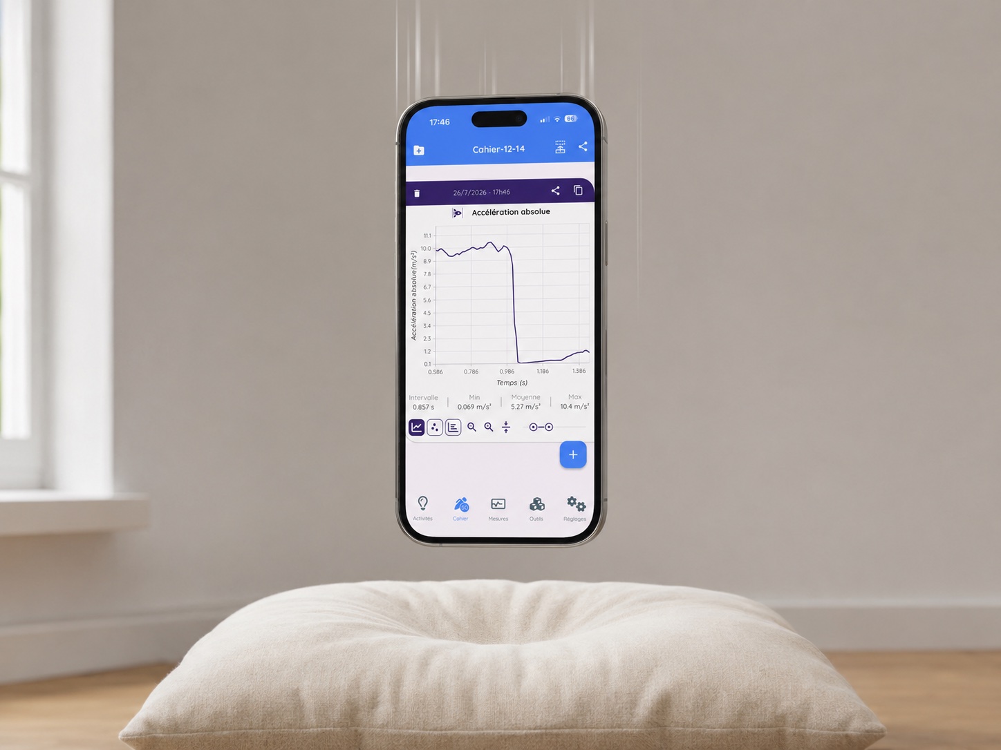
During the fall (with air drag neglected), the absolute acceleration tends toward zero: no contact force acts anymore, and the proof mass floats. This is the signature signal of weightlessness, the one exploited by laptop drop sensors and by parabolic flights.

Linear acceleration, on the other hand, may then show a magnitude close to g: the operating system keeps estimating a gravity vector and subtracts it from a raw measurement that has gone to zero, so the result of the computation is the opposite of the estimated gravity. But because it is a computed quantity, its exact behavior during the fall depends on the device’s processing (filtering, duration of the fall, fusion algorithm, any rotation of the phone): the magnitude is close to g only if the gravity estimate stays stable. The genuinely robust observation is therefore the disappearance of the raw measurement. Physically, all of this is consistent: the phone really does accelerate toward the ground at about 9.81 m/s² in the lab frame.

The two quantities describe the same event from two complementary points of view: absolute acceleration tells you what the device feels, linear acceleration describes its motion. To demonstrate weightlessness in class, display absolute acceleration: during the fall, the curve drops sharply toward zero.

4.5 Which instrument should you choose?

Experiment	Recommended quantity	Why
Static tilt	Absolute acceleration (or estimated gravity)	Uses the projection of the vertical
Free fall	Absolute acceleration	Demonstrates weightlessness
Elevator acceleration	Both absolute and linear, for comparison	Shows apparent weight
Vehicle braking	Linear acceleration	Removes the main effect of gravity
Pendulum	Absolute or linear, depending on the setup	Depends on the phone’s orientation
Circular motion	Absolute acceleration + gyroscope	Lets you test a_c = Rω²
Vibration	Appropriate component or magnitude	Periodic signal
Displacement by integration	Linear, with strong reservations	Drift accumulates fast (Section 9)

5. How does a MEMS gyroscope work?

5.1 From the mechanical gyroscope to the MEMS gyroscope

The word “gyroscope” comes from the nineteenth-century rotor instruments: a rapidly spinning wheel whose axis keeps its orientation, used for navigation. A smartphone gyroscope contains no spinning wheel at all: it is a MEMS sensor built on an entirely different principle, detecting the Coriolis force on a vibrating microstructure. Only the name survives.

5.2 A vibrating structure sensitive to the Coriolis force

Inside the sensor, a microstructure is driven into rapid vibration along a fixed direction. When the device rotates, the Coriolis force deflects that vibration perpendicular to its motion. This tiny transverse displacement is detected electrically (through a change in capacitance, as in the accelerometer), and its amplitude is proportional to the rate of rotation: from it the sensor derives the angular velocity.

5.3 Three axes of rotation

Like the accelerometer, the gyroscope supplies three components: ω_x, ω_y, and ω_z, the rates of rotation about the phone’s three axes, usually expressed in radians per second. The magnitude is computed the same way:

|ω⃗| = √(ω_x² + ω_y² + ω_z²)

with |ω⃗| and its components in rad/s.

5.4 The positive sense of rotation

The sign of each component follows the right-hand rule: with the thumb pointing along the positive direction of the axis, the curled fingers give the positive sense of rotation. With the phone flat, a counterclockwise rotation viewed from above therefore gives a positive ω_z in the usual convention. A quick test — turning the phone slowly each way while watching the sign — removes any ambiguity on your own device.

5.5 The gyroscope does not measure an angle directly

The gyroscope supplies an angular velocity, not an orientation. To get an angle, you have to accumulate the rotations over time. Over a small interval:

Δθ ≈ ω Δt

and, for rotation about a fixed axis:

θ(t) = θ(t₀) + ∫[t₀→t] ω(τ) dτ

with θ in radians, ω in rad/s, and t in seconds.

Going further. This integration holds only for rotation about a fixed axis. In three dimensions, you cannot reconstruct orientation by integrating ω_x, ω_y, and ω_z separately, because successive rotations do not commute. The operating system then uses suitable representations, such as rotation matrices or quaternions.

An immediate consequence: any bias in angular velocity, however tiny, accumulates under integration. An offset of 0.01 rad/s produces an angular error of 0.6 rad (about 34°) after one minute. This is why an orientation computed from the gyroscope alone drifts, and why the operating system continuously corrects it using other sensors.

6. How the smartphone estimates its orientation

6.1 What the accelerometer contributes

At rest or in slow motion, the measured vector is vertical: it is carried by the normal force from the support, and therefore lies along the local vertical. The accelerometer then provides a reliable vertical reference. The sign of the displayed vector, on the other hand, is a platform-specific convention, which has no bearing on its use as a direction reference. This reference degrades as soon as the device undergoes appreciable acceleration from motion, which mixes into the response to the support.

6.2 What the gyroscope contributes

The gyroscope tracks rotations quickly and finely, while being ideally insensitive to translational motion (far more so than an accelerometer). But its integration drifts (5.5): excellent in the short term, it loses the reference over the long term.

6.3 The role of the magnetometer

The magnetometer can supply a heading reference (the direction of Earth’s magnetic field), stable over time. It is, however, disturbed by magnets, metal structures, and nearby electronics: its reference is durable but locally fragile.

6.4 Sensor fusion

The operating system combines these three complementary sources: the accelerometer’s vertical (correct in the long run, scrambled during motion), the gyroscope’s rotation (precise in the short term, drifting), and the magnetometer’s heading (stable but subject to disturbance). This fusion produces the computed quantities: the estimated gravity vector, the device’s orientation, and the linear acceleration. The exact algorithms depend on the operating system and the manufacturer; it would be inaccurate to claim that one single method is used on all devices. The techniques go by names such as complementary filter or Kalman filter, mentioned here without further development.

6.5 Why a tilt measurement goes wrong during motion

The accelerometer measures only one vector: the sum of the response to the support and the effects of the motion. With no additional information, it cannot separate the two. A tilted, stationary phone and an upright phone accelerating horizontally can produce similar readings. This is why accelerometer-based tilt measurements are reliable only in static or quasi-static conditions, and why the system needs the gyroscope to track orientation during motion.

7. Sampling rate and digital acquisition

7.1 What is a sample?

A sample is a time-stamped measurement point: a value together with the instant it was acquired. A recording is a sequence of samples, and the whole analysis (graph, period, frequency) rests on these value–time pairs.

7.2 Requested rate versus actual rate

The sampling rate is the number of samples acquired per second. It depends on the phone model, the operating system, the sensor in question, processor load, the app’s settings (FizziQ lets you adjust the acquisition rate in its settings), and power-saving policies. No universal value applies to all smartphones: the typical order of magnitude runs from a few tens up to about a hundred hertz for motion sensors, but the only reliable value is the one you measure on your own device.

7.3 Measuring the sampling rate from the timestamps

Exporting the data (CSV or Python in FizziQ) gives access to the instants tᵢ of each sample. Compute the intervals:

Δtᵢ = tᵢ₊₁ − tᵢ

then the effective rate, from the mean interval:

f_e ≈ 1/Δt̄

or directly over the whole recording:

f_e ≈ (N−1)/(t_N − t₁)

with N the number of samples, t₁ and t_N the instants of the first and the last. This is a simple, instructive measurement, worth doing once per device.

7.4 Slightly irregular sampling

The intervals Δtᵢ are not rigorously constant: the operating system may delay or batch data deliveries. These small irregularities are inconsequential for most classroom experiments, but they are a reminder that a stated rate is an average, not a perfect clock.

7.5 Which vibrations can you observe?

A signal is faithfully reproduced only if the sampling is substantially faster than its variations. The Nyquist criterion sets the theoretical limit: the sampling rate f_e must exceed twice the frequency of the phenomenon; equivalently, the highest usable frequency is f_e/2. So for a motion sensor sampled between 50 and 100 Hz — the usual range for accelerometers and gyroscopes — the theoretical Nyquist limit falls between 25 and 50 Hz depending on the device, and the comfortable range for quantitative analysis is far lower.

Two regimes must be distinguished. Below that limit, the closer the phenomenon’s frequency comes to it, the less faithful the shape of the signal: ten or so points per period describes a phenomenon well, two or three give only a silhouette. Above the limit, the problem changes in kind: the phenomenon is not merely poorly described, it appears at a false, lower frequency — perfectly legible and perfectly misleading. This is aliasing, and nothing in the curve flags it: the only simple defense is to repeat the measurement at a different sampling rate and check that the result does not change.

Note, though, that MEMS accelerometers often include an analog low-pass filter ahead of digitization, which partially attenuates this aliasing: the clear-cut case described here is somewhat less common than it might seem, which makes the rate-change test all the more useful without turning it into a constant worry. The sensor’s own bandwidth adds a further limit. For fast vibrations, the microphone — sampled far more rapidly — takes over.

8. Accuracy, noise, bias, drift, and saturation

Five distinct notions, often confused, describe the limits of these sensors.

8.1 Resolution

The smallest numerical change observable in the data. It depends on the component and the digitization chain, and says nothing about accuracy.

8.2 Noise

The fast, random fluctuations visible when the phone is at rest: the acceleration curve is never a perfect straight line. Noise sets the practical limit on the smallest detectable variations.

8.3 Bias

A nonzero mean value where the quantity should be zero: for example a mean linear acceleration of 0.03 m/s² at rest, or a nonzero angular velocity on a stationary phone. Bias does not go away by averaging longer.

8.4 Drift

The slow evolution of the bias with time or temperature. It matters especially for the gyroscope, whose integration turns the slightest drift into a growing angular error.

8.5 Saturation

Every sensor has a maximum measurable value. Beyond it, the reading flattens out: the peaks of a violent impact are clipped and the measurement loses its meaning. Repeated flattening at the same value is the telltale sign of saturation.

8.6 Filtering and smoothing

The sensor itself and the operating system may filter the signal before passing it on: a filtered signal is easier to read but responds with a lag and attenuates peaks. This filtering, which you undergo rather than control, must be distinguished from the smoothing applied afterward to the data in the experiment notebook, which FizziQ offers as modeling options (linear interpolation, quadratic smoothing). This second kind of smoothing does not alter the recorded data: it merely proposes a representation of it. In both cases the same rule holds: a smoothed signal is not necessarily a more accurate one.

8.7 Differences between smartphones

Performance varies with the component installed, the measurement range chosen by the manufacturer, the sampling rate, the filters, the operating system, and the fusion algorithm. Alongside bias (an additive offset), a scale factor error (a multiplicative discrepancy between the true value and the displayed one) directly explains why one phone reads 9.7 and another 9.9 m/s² for the same magnitude at rest: this is the observation behind Experiment 4. No generic accuracy figure can be quoted for “smartphones” in general: two devices give different results, which makes this a good vehicle for discussing reproducibility.

8.8 Characterizing your own device

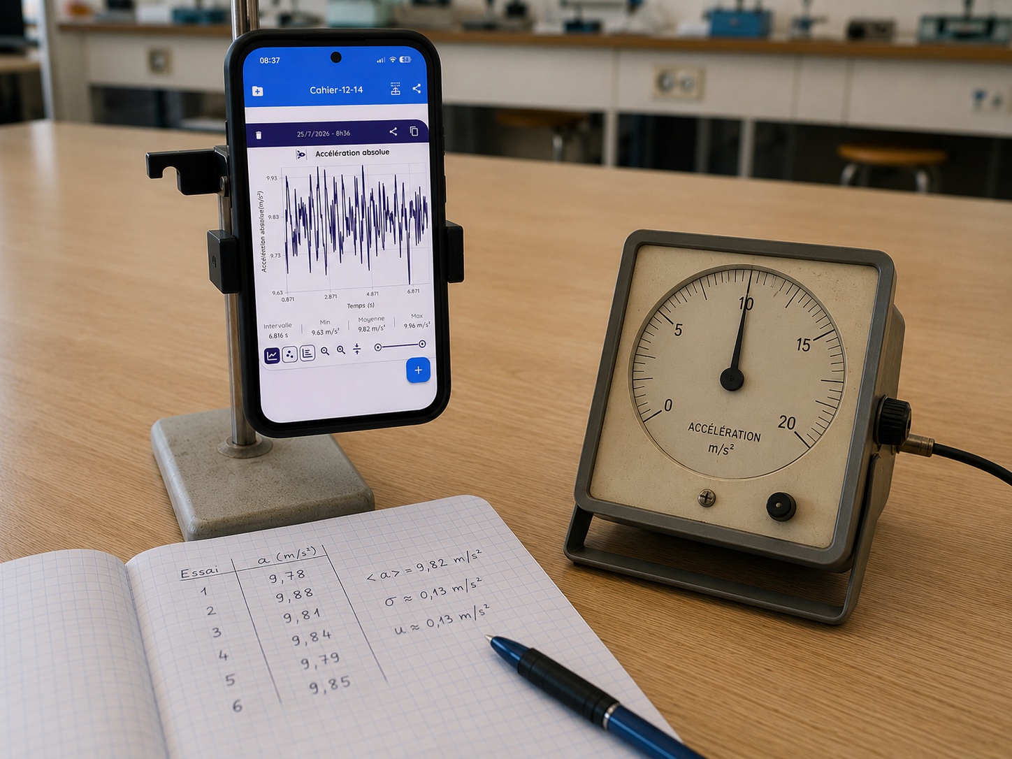
A classroom method in seven steps: (1) hold the phone perfectly still; (2) record several seconds of absolute acceleration and angular velocity; (3) compute the mean, minimum, maximum, and standard deviation; (4) repeat in several orientations; (5) compare the mean acceleration magnitude with a reasonable local value of g; (6) look for any bias (nonzero linear acceleration or angular velocity at rest); (7) document the phone model and the conditions. The full analysis procedure (spread, standard uncertainty, calibration) is covered in the guide to measurement uncertainty with a smartphone on fizziq.org.

9. Can you compute velocity and position from the accelerometer?

9.1 From acceleration to velocity

Mathematically, velocity is obtained by integrating acceleration:

v(t) = v(t₀) + ∫[t₀→t] a(τ) dτ

9.2 From velocity to position

And position by integrating velocity:

x(t) = x(t₀) + ∫[t₀→t] v(τ) dτ

These two relations are written here for motion along a single axis; in the general case they are vector relations for v⃗(t) and r⃗(t), and the acceleration must first be expressed in a fixed frame, which requires knowing the phone’s orientation at every instant.

9.3 Why do the errors pile up?

In theory, then, two integrations suffice to reconstruct a trajectory. In practice, the method fails quickly. A numerical example shows why. Suppose a very modest residual bias of 0.05 m/s² in the linear acceleration of a stationary phone. After integration, that bias produces a false velocity growing linearly: 3 m/s after one minute. The second integration turns that false velocity into a false position growing as the square of time: ½ × 0.05 × 60² = 90 meters of error in one minute, for a phone that never moved. Noise adds its own contribution, but bias dominates: integration amplifies systematic errors.

9.4 When is integration still useful?

It retains value in well-defined cases: very short motions (a few seconds); motions known to start and end at rest, which allows the drift to be corrected; qualitative comparisons; processing with explicit bias correction; and above all, the pedagogical exercise of demonstrating the drift itself (Experiment 12). You should never leave the impression that an ordinary smartphone can accurately reconstruct a long-duration trajectory from its accelerometer alone: professional inertial navigation systems use incomparably more stable sensors, and continuously correct them against other references.

10. Accessible motions and models

10.1 Straight-line motion

Starts, stops, and changes of speed can be read directly from the linear acceleration, provided you fix the phone’s orientation and identify the axis of motion. The phases show up on the graph: a positive peak at the start, a plateau near zero at constant velocity, a negative peak on braking.

10.2 Vertical motion and the elevator

In an elevator, the vertical absolute acceleration reflects the apparent weight: slightly greater than g when starting upward, equal to g while rising at constant velocity, less than g while slowing. A note on vocabulary: the sensor does not measure weight, it measures contact force per unit mass; the link to the sensation of heaviness or lightness is made through Newton’s second law.

10.3 Oscillations and the pendulum

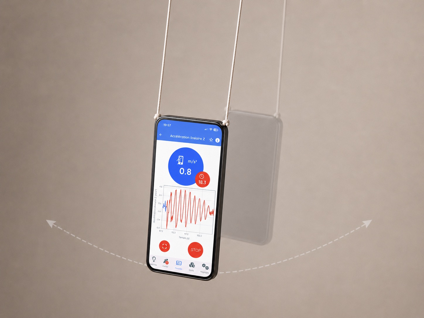
A phone suspended from, or attached to, a pendulum produces a periodic signal from which you measure the period T, hence the frequency f = 1/T. The shape of the signal depends on the phone’s orientation and on the quantity chosen; the period measurement, by contrast, is robust: count several oscillations and divide the total time.

10.4 Vibration

With the phone resting on a vibrating surface (a speaker, a machine, a table), the time signal reveals the period of the vibration and its amplitude, within the sampling limits of Section 7.

10.5 Circular motion

Pairing the accelerometer with the gyroscope is especially useful for this motion. For an object in uniform rotation at a distance R from the axis:

v = Rω and a_c = v²/R = Rω²

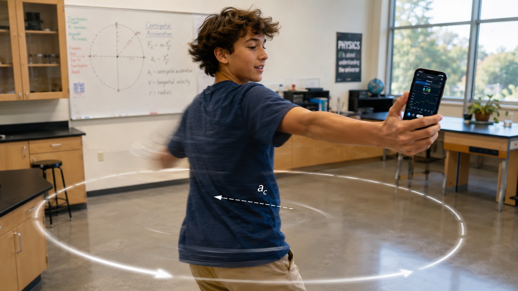
with v the tangential speed (m/s), ω the angular velocity (rad/s), R the radius (m), and a_c the centripetal acceleration (m/s²), directed toward the axis. The gyroscope gives ω. For a_c, take care: if the axis of rotation is vertical, the magnitude A of the absolute acceleration mixes the radial component (≈ a_c) with the vertical component (≈ g), so that A = √(a_c² + g²). You must therefore either use the accelerometer component along the radial axis directly (|a_radial| ≈ Rω²), or remove the vertical contribution from the magnitude using a_c ≈ √(A² − g²). Both relations assume uniform rotation: as soon as the rate of rotation changes, a tangential component is added and corrupts the correction. This is why readings should be taken during the steadiest phases of rotation, not during spin-up or slow-down. You then have two distinct measurements (ω and a_c) for two quantities linked by the model, which makes it possible to test the relation experimentally (Experiment 11).

10.6 Tilt

In static conditions, gravity projects onto the phone’s axes. Consider a phone tilted by an angle θ from the horizontal, rotated about its y-axis, with the x-axis placed along the line of steepest slope and the z-axis perpendicular to the screen. Depending on the device’s sign convention, the measured components then satisfy:

|a_x| = g |sin θ| and |a_z| = g |cos θ|

and the angle follows, across the whole measurement range and independently of the value of g, from:

θ = atan2(a_x, a_z)

These relations make sense only when accompanied by a diagram that precisely defines the axis of rotation, the origin of the angle, and the sign of each component (a diagram is indispensable here); the exact signs must be checked experimentally on the device in use, and the whole treatment remains restricted to static situations (6.5).

11. Using FizziQ to record and analyze the data

In FizziQ, the motion sensors are reached from the Instruments tab: there you choose absolute or linear acceleration (per X, Y, Z component or as a magnitude, in m/s²) and the gyroscope (rate of rotation per component or as a magnitude). The measurement screen shows the live value and its graph; recording adds the data series to the experiment notebook, where it can be viewed, zoomed, and annotated. Duo mode lets you display two instruments at once — for example acceleration and angular velocity for circular motion. The app settings let you adjust the sampling rate and the signal smoothing. Data can be exported as CSV or Python for processing in a spreadsheet or in code, and shared between devices by QR code.

Goal	FizziQ instrument	What to look at	Main limitation
Check the axes	Absolute acceleration X, Y, or Z	Which component carries g in each orientation	Device-specific sign conventions
Demonstrate weightlessness	Absolute acceleration (magnitude)	The plunge toward zero during the fall	Very short fall duration
Study a motion (braking, starting)	Linear acceleration	Component along the axis of motion	Residuals during rotations
Measure an oscillation period	Acceleration (absolute or linear)	Periodicity of the signal	Phone orientation
Measure a rate of rotation	Gyroscope	Component along the rotation axis, or magnitude	Saturation at fast rotation
Test a_c = Rω²	Accelerometer + gyroscope (Duo mode)	a_c and ω simultaneously	Mounting and centering of the phone
Characterize noise and bias	Any instrument, device at rest	Mean and standard deviation at rest	Depends on the device model

---

Lab Safety

Read before running any experiment. Protect the smartphone against impact (case, padding). Secure the device firmly in any circular motion, and check the strength of all strings, stands, and fasteners. Avoid fast rotations. Do not throw the phone. Never place anyone in the path of a moving device. Do not handle a smartphone while driving: in-vehicle experiments are run by a passenger. Keep drop experiments to very small heights, over a cushion, a padded box, or an equivalent. Stop an experiment immediately if the setup becomes unstable.

---

Twelve Experiments with the Accelerometer and Gyroscope

The twelve experiments below go deeper into the use of the accelerometer and gyroscope. Complementary activities on video analysis, GPS, and sound appear in their respective parts. They are ordered by increasing difficulty, and the safety box above applies to all of them.

Experiment 1: Find the smartphone’s three axes

Scientific question: How do the components reflect the device’s orientation? Level: Middle school, grades 9–10. Time: 15 min. Materials: One smartphone. FizziQ instrument: Absolute acceleration X, then Y, then Z. Setup: Phone placed in turn flat, upright, on its edge, then flipped over. Procedure: In each position, record which component carries the value close to 9.8 m/s², and its sign. Measured quantities: Three acceleration components. Representation: Position-versus-component table. Calculation or model: Projection of the vertical onto the axes. Expected result: One dominant component per position, changing sign when the phone is flipped. Precautions: Stable surface. Main source of uncertainty: Imperfectly aligned positions. Interpretation: The sensor’s frame is fixed to the device. Related resource: Glossary entry Accelerometer.

Experiment 2: Check that the magnitude stays close to g

Question: What happens to the magnitude when you tilt the device? Level: Grades 9–10. Time: 20 min. Materials: One smartphone. Instrument: Absolute acceleration, components then magnitude. Setup: Phone stationary, tilted slowly by hand or on shims. Procedure: Record components and magnitude for several tilt angles. Quantities: Components and magnitude. Representation: Table, or curves during a slow tilt. Model: |a⃗| = √(a_x² + a_y² + a_z²). Expected result: Variable components, magnitude stable and close to g. Precautions: Move very slowly to stay quasi-static. Main uncertainty: Small accelerations from the hand movement. Interpretation: The physical situation has not changed; only its projection has rotated. Resource: Article Seven Experiments on Gravity.

Experiment 3: Turn the smartphone into an inclinometer

Question: Can you measure an angle with the accelerometer? Level: Grades 10–11. Time: 30 min. Materials: Smartphone, adjustable ramp, protractor for checking. Instrument: Absolute acceleration along one axis. Setup: Phone resting on the ramp, chosen axis along the line of steepest slope. Procedure: For several tilt angles, record two components (the one in the plane of the screen along the line of steepest slope, and the one perpendicular to the screen), compute the angle from θ = atan2(a_x, a_z), and compare with the protractor. Quantities: Acceleration component, angle. Representation: Measurement-versus-protractor table. Model: Projection of g⃗ (diagram indispensable). Expected result: Agreement to within a few degrees. Precautions: Strictly static conditions. Uncertainty: Sensor bias and zero setting. Two formulas can be used to exploit the components, and they do not degrade the same way with angle. With the single-component formula a_axis = g sin θ, which is more intuitive, an error of 0.05 m/s² in the measurement translates into an angular error of about 0.3° near the horizontal, 0.6° at 60°, but 1.7° at 80° and 3.4° at 85°: the component varies less and less with angle as you approach the vertical. The two-component formula, by contrast, keeps a constant sensitivity and stays usable across the whole range. Interpretation: Static tilt follows from the sensed vertical. Resource: FizziQ activity Inclined Plane: Components of Weight.

Experiment 4: Estimate g with the smartphone

Question: What value of g does a smartphone give? Level: Grades 10–12. Time: 45 min. Materials: One or more smartphones. Instrument: Absolute acceleration (magnitude), with recording. Setup: Device stationary in several orientations. Procedure: Record 30 s per orientation, compute the mean and standard deviation, compare across orientations and across devices. Quantities: Magnitude of the acceleration. Representation: Table, histogram. Calculation: Mean, spread. Expected result: Values close to 9.8 m/s², with differences between orientations and between devices. Precautions: Do not present the result as a precise metrological determination of g. Uncertainty: Calibration bias specific to each device. Interpretation: A discussion of accuracy, precision, and bias. Resource: Guide Understanding Measurement Uncertainty.

Experiment 5: Demonstrate weightlessness in free fall

Question: What does an accelerometer read while falling? Level: Grades 11–12. Time: 45 min. Materials: Smartphone, thick cushion or padded box. Instrument: Absolute acceleration (magnitude), with recording; then compare with linear acceleration. Setup: A vertical drop from a very small height (a few tens of centimeters) above the landing pad. Procedure: Set the sampling rate to the maximum available in the settings, start recording, release (do not throw) the phone, then analyze the curve. Quantities: Acceleration magnitude versus time. Representation: Time graph. Model: Weightlessness during the fall; fall duration t = √(2h/g). Expected result: A plunge of the absolute acceleration toward zero during the fall, and a spike on landing. Precautions: Minimal height, soft landing, never a throw. Uncertainty: The number of points available during the fall. A 30 cm drop lasts about 0.25 s, which is a dozen points at 50 Hz and about 25 points at 100 Hz. The weightlessness plateau is therefore short and you have to zoom in to see it. After that come air drag and the detection of the start and end instants. Interpretation: The sensor no longer feels anything: this is local weightlessness. Resource: FizziQ activity Weightlessness and Free Fall.

Experiment 6: Study an elevator starting and stopping

Question: How does apparent weight change in an elevator? Level: Grades 11–12. Time: 30 min on site. Materials: Smartphone, elevator. Instrument: Vertical absolute acceleration, with recording; comparison with linear acceleration is possible. Setup: Phone flat on the floor of the car. Procedure: Record a complete trip, then identify the start, the near-constant-velocity phase, the slowing phase, and the stop. Quantities: Vertical acceleration. Representation: Time graph annotated with the phases. Model: Apparent weight, Newton’s second law. Expected result: A bump at the start, a plateau at g, a dip while slowing (going up), and the reverse going down. Precautions: Be considerate of other passengers. Uncertainty: Vibration of the car. Interpretation: During the constant-velocity phase, the accelerometer reads the same value as at rest: it cannot tell you the velocity. Resource: FizziQ activity Einstein’s Elevator: The Equivalence Principle.

Experiment 7: Measure braking or acceleration in a vehicle

Question: What acceleration does a vehicle undergo when starting or braking? Level: Grade 12. Time: 45 min. Materials: Smartphone in a mount (car phone holder), vehicle, a driver and a passenger acting as experimenter. Instrument: Linear acceleration along the axis of motion. Setup: Phone firmly mounted, axis aligned with the direction of travel. Procedure: The passenger (never the driver) records several ordinary starts and stops. Quantities: Longitudinal acceleration. Representation: Time graph. Calculation: Peak values, orders of magnitude (1 to 3 m/s² in normal use). Expected result: Clearly identifiable positive and negative peaks. Precautions: Normal driving, no handling by the driver; results presented as pedagogical, not as a road-safety assessment. Uncertainty: Orientation of the mount (a tilt of just 5° reinjects g·sin 5° ≈ 0.85 m/s², a substantial fraction of the useful signal), road grade, vibration. Interpretation: A direct reading of the phases of straight-line motion. Resource: Guide Doing Physics with a Smartphone.

Experiment 8: Study the oscillations of a pendulum

Question: What is the period of a pendulum? Level: Grades 11–12. Time: 1 hr. Materials: Smartphone, two strings of equal length, and a support (rod, ring stand, or the back of a chair) that lets you attach them a few centimeters apart; tape measure. Instrument: Gyroscope, the component perpendicular to the plane of oscillation — the phone’s X-axis if the strings are attached at its two upper corners and it swings screen-forward. With recording. Absolute acceleration (preferably its magnitude, or its component along the string) as a second instrument for comparison. Setup: The phone hangs from two strings, and the plane of oscillation must be perpendicular to the line joining the two attachment points, like the two ropes of a playground swing. This arrangement serves two purposes. First, the two strings prevent the phone from twisting about the vertical, which a single-string suspension does not guarantee: the rotation therefore stays on a single sensor axis. Second, they let the phone tilt along with the pendulum, which is essential since the gyroscope measures only changes in orientation. Take care not to place the strings one in front of the other within the plane of oscillation: the setup would become a deformable parallelogram, the phone would move without ever rotating, and the gyroscope would record nothing. A ten-second trial settles the question before you begin: the gyroscope signal must oscillate clearly. Use a moderate amplitude, around twenty degrees. Procedure: Start recording, let it swing, and measure on the gyroscope signal the time for ten complete oscillations, then divide by ten. Repeat with the absolute acceleration and compare the two periods you read. Quantities: Angular velocity, acceleration, period. Representation: Zoomed time graph, with the two signals overlaid if Duo mode is available. Model: For small amplitudes, T = 2π√(L/g), if the setup approximates a simple pendulum. Expected result: The gyroscope gives a sinusoidal signal of period T, maximum as the pendulum passes through the vertical and zero at the turning points. The magnitude of the absolute acceleration, or its component along the string, has period T/2: it reaches a maximum at every pass through the vertical, whichever way the pendulum is moving. This is the most instructive result of the experiment. Precautions: Attachment suited to the mass of the phone; no one in the path of the swing. Uncertainty: The main source is the setup itself, which is not a simple pendulum — the phone is not a point mass and the length L stays ill-defined to within a few centimeters. The phone can also rock slightly about the line of its two attachment points, superimposing a faster ripple on the signal; moving the attachment points closer to the center of the device reduces it. The departure from the small-amplitude formula comes far behind: for an amplitude of 20°, the correction to the period is only 0.8%. Interpretation: A suspended phone experiences only one contact force, the tension in the string. The specific force along the string is g(3 cos θ − 2 cos θ₀): it depends only on |θ|, so it repeats twice per period. The gyroscope, which measures θ̇, does distinguish the two directions of travel: it is the one that gives T directly. Confusing the two signals would halve the period, and therefore divide the inferred length by four. That the phone really does tilt with the string has a simple explanation: in the pendulum’s frame, the specific force points along the string, so the phone’s center of mass, hanging below the line of its two attachment points, continuously aligns itself with that direction — exactly like the seat of a playground swing. Resource: FizziQ activity Period of a Pendulum.

Experiment 9: Measure the frequency of a slow vibration

Question: At what frequency does this system oscillate, and how do you know the measurement is trustworthy? Level: Grades 11–12. Time: 45 min. Materials: Smartphone and a slow vibration source, your choice of: a spring with the phone hanging from it (about 1 to 3 Hz), or a flexible strip clamped at the edge of a table with the phone attached to its free end (a few hertz). Rule out rotating machines such as a washing machine on spin cycle: the phone would simply be set on top, and could fall, and the rotation frequency there exceeds the range the accelerometer reproduces faithfully. Instrument: Absolute acceleration along the axis of oscillation, with recording. Setup: Phone rigidly attached to the vibrating part, never simply resting on a slippery surface. Procedure: First set the sampling rate to the maximum available in the settings; record about ten seconds; zoom in, measure the duration of several periods, and compute f = 1/T. Then repeat the same recording at a lower sampling rate and compare the two results. Quantities: Period, frequency, effective sampling rate. Representation: Time-domain oscillation. Model: Periodic signal; Nyquist criterion. Expected result: A stable frequency, identical at both sampling rates. If it changes when you change the sampling, the value you read is not the source’s: this is aliasing, and the source is vibrating too fast for this sensor. Precautions: Secure attachment, no violent vibration, do not balance the phone on a running appliance. Uncertainty: Number of points per period; reading the instants off the graph. Interpretation: A smartphone accelerometer sampled at a few tens of hertz faithfully reproduces only phenomena much slower than half its sampling rate. The consistency test by changing the sampling rate is the only simple check available to the experimenter. Resource: Guide Measuring and Analyzing Sound, for higher frequencies, where the microphone takes over.

Experiment 10: Measure a rate of rotation with the gyroscope

Question: How fast is this device rotating? Level: Grades 11–12. Time: 45 min. Materials: A slow turntable, or a swivel chair used with care. Instrument: Gyroscope (vertical-axis component, or magnitude). Setup: Phone fastened at the center of the device. Procedure: Rotate steadily and slowly; record; in parallel, count the turns and time the period. Quantities: Angular velocity, period, number of turns. Representation: Graph of ω. Model: ω = 2π/T. Expected result: Agreement between the measured ω and the computed 2π/T. Precautions: Slow rotations, device well secured. Uncertainty: Irregularity of the hand-driven rotation. Interpretation: The gyroscope measures directly what the stopwatch gives only indirectly. Off-center placement of the phone does not affect the measured rate of rotation ω (a rotating rigid body turns at the same angular velocity at every point), but it does change the centripetal acceleration a_c: that is the starting point of Experiment 11. Resource: Glossary entry Gyroscope.

Experiment 11: Test the relation a_c = Rω²

Question: Does centripetal acceleration follow the circular-motion model? Level: Grade 12. Time: 1 hr 30. Materials: A closed, secured device — for example an adapted salad spinner — plus padding. Instrument: Accelerometer and gyroscope, in Duo mode if possible. Setup: Phone completely immobilized in the basket, at a measured distance R from the axis (with the sensor’s position taken to be at the center of the device). Procedure: Spin at several moderate rates; for each one, record ω and the centripetal acceleration, using the accelerometer’s radial component or, if only the magnitude A is available (vertical rotation axis), computing a_c ≈ √(A² − g²); measure R. Quantities: ω, a_c, R. Representation: Graph of a_c versus ω². Model: a_c = Rω²; the expected slope is R and the intercept should be zero. A nonzero intercept signals a faulty correction for g or an off-center phone: this is a validity test at least as instructive as the slope. Expected result: A straight line whose slope is close to the measured radius. Precautions: Moderate speeds, lid closed, stop immediately if the setup shifts. Check that the phone is not tilted inside the basket: the magnitude-based correction assumes a horizontal radial axis. Take readings during the steadiest phases of rotation, not during spin-up. Uncertainty: The exact position of the sensor inside the phone, and hence R; the correction for g if you start from the magnitude; accelerometer saturation at high speeds. With R = 7 cm, the centripetal acceleration reaches 20 m/s² at just 2.7 revolutions per second and exceeds 60 m/s² at 5 revolutions per second: depending on the device’s measurement range, the high points may be clipped. Flattening of the signal at a constant value is the telltale sign of saturation; those points must be excluded from the regression. Interpretation: Two distinct measurements (accelerometer and gyroscope) confirm the same model. Resource: FizziQ activity Centripetal Acceleration: The Salad Spinner.

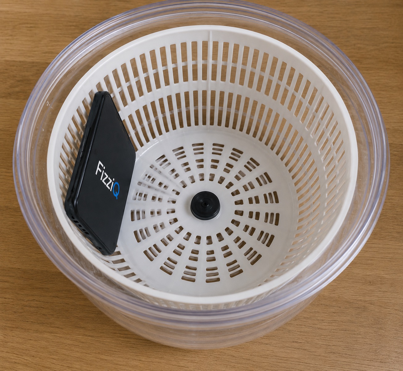
Experiment 12: Demonstrate the drift of integration

Question: Can you recover velocity by integrating acceleration? Level: Grade 12, first-year college. Time: 1 hr. Materials: Smartphone, spreadsheet or Python. Instrument: Linear acceleration, recorded on a perfectly stationary phone; CSV or Python export. Setup: Device set down, untouched, for one to two minutes. Procedure: Export the data and compute the reconstructed velocity by cumulative numerical integration (vᵢ₊₁ = vᵢ + aᵢ Δtᵢ). Quantities: Acceleration, integrated velocity. Representation: Graph of the computed velocity versus time. Model: Integration; the effect of a constant bias (Section 9.3). Expected result: A nonzero velocity appears and grows, even though the phone never moved. Precautions: None (a desk experiment). Uncertainty: Sensor bias and noise — precisely what the experiment is meant to reveal. Interpretation: An explicit demonstration of the limits of inertial navigation with a consumer-grade sensor. Resource: Guide Understanding Measurement Uncertainty.

---

Part 3: Studying Motion by Video Analysis

The accelerometer and gyroscope measure the motion of the smartphone itself. That method works especially well when the device can be attached to the object under study. When the smartphone has to stay still and observe another object, video analysis is generally the better fit: it reconstructs the object’s trajectory in the lab frame.

You film (or import) a video, then reconstruct the object’s complete trajectory, frame by frame. For a full overview, see the complete guide to video analysis and chronophotography.

The “Kinematic Analysis” instrument and its two modes

FizziQ offers a dedicated instrument with two complementary modes:

Mode	Medium analyzed	Quantities measured
Video kinematics	A video	Position (x, y), velocity, acceleration
Chronophotography	A photo	Position (x, y), velocity (Vx, Vy, V), acceleration (Ax, Ay, A), rotation (α), energies (KE, PE, ME)

Chronophotography mode therefore goes all the way to an energy budget, which is ideal for illustrating conservation of mechanical energy. Note, though, that the energy calculation rests on two choices made by the experimenter, not on measurements: entering the object’s mass, and choosing a conventional zero for the potential energy. To go further with this approach, see Using Chronophotography in Lab.

The three-step procedure

1. Set the scale: calibrate the video against an object of known length visible in the frame, to convert pixels into meters.
2. Track the motion: frame by frame, click manually on the object’s position. This manual tracking demands care, but it keeps the student an active participant in the measurement.
3. Use the results: FizziQ computes the quantities and adds them to the experiment notebook as tables and graphs, exportable as CSV or Python.

Positions come directly from the tracking. Velocities and accelerations are then computed from those positions: they are therefore more sensitive to tracking errors, acceleration especially.

The user guide for the kinematics tool covers each operation in detail.

Getting a good video

The quality of the results depends directly on the shot: film perpendicular to the plane of the motion to limit parallax, and ensure good lighting and sharp contrast. Tracking uncertainty stays at a few pixels, and the time resolution is set by the video’s frame rate. Our 7 Tips for a Good Video will steer you past the most common pitfalls. No equipment to film? The FizziQ video library supplies ready-to-track footage.

A special precaution applies to slow-motion video. Most phones record it at a high frame rate, then export it in a file played back at 30 frames per second, with time stretched out. The interval between two frames of the file then no longer corresponds to 1/30 s of real time, but to 1/120 or 1/240 s. If that true frame rate is not taken into account, every velocity and acceleration computed is wrong by a factor of 4 or 8, with nothing on the graph to signal it. The simplest check is to film a free fall and verify that the acceleration you get really is about 9.8 m/s².

When should you choose video? When the smartphone cannot be attached to the object, when you want a trajectory in the lab frame, or when you want to view position, velocity, and acceleration at the same time.

Related FizziQ activities

Video analysis complements the inertial sensors: it lets you reconstruct the trajectory of an object separate from the smartphone and study large-amplitude motion in the lab frame. A few ready-to-run activities:

• Measuring g by Video Analysis and Free Fall: Measuring g;
• Parabolic Trajectory in Basketball and Taking a Shot in Soccer;
• Energy Budget of a Pole Vault and A Skier’s Speed on Video.

Sports become a prime testing ground, as our selection of 12 Sports to Study with a Smartphone shows.

---

Part 4: Studying Displacement with GPS

GPS turns your smartphone into a position-tracking beacon. In FizziQ, the GPS instrument supplies several data streams at once: latitude (−90° to +90°), longitude (−180° to +180°), altitude (in meters, with a reference that depends on the platform — see below), GPS speed (in m/s or km/h), and GPS accuracy (a horizontal confidence radius, in meters, and not a guaranteed error bound). It is a valuable tool for taking physics out of the lab and studying motion on a large scale.

Which quantities to record, and how to use them

All of these are recorded in the experiment notebook, second by second, and can then be exported as CSV or Python. From the sequence of successive positions (latitude, longitude), you reconstruct the path and compute the distance traveled. The average speed then follows simply as that distance divided by the elapsed time. The instantaneous speed is supplied directly by the smartphone’s location service. Cross-referencing these lets you compare, for instance, instantaneous and average speed over the same trip.

A major limitation: the 1 Hz update rate

GPS records only about one point per second (1 Hz). That is its great limitation: fast or small-scale motion is out of reach, because between two points the object has already moved a long way. GPS is therefore reserved for slow, large-scale motion: walking, running, cycling, hiking, or traveling by car or boat. For laboratory-scale motion, prefer the accelerometer or video analysis.

Accuracy, altitude, and conditions of use

Position accuracy is often several meters and depends heavily on conditions: clear sky, no nearby buildings. This is why GPS is used outdoors, after a short period for the signal to stabilize.

GPS altitude is markedly less reliable than latitude and longitude, for two distinct reasons that are worth keeping apart. The first is geometric: vertical position is intrinsically less well determined by the satellites than horizontal position. The second has to do with the reference chosen. Android returns altitude above the WGS84 ellipsoid, a mathematical model of the Earth, while iOS returns an altitude referenced to mean sea level. The two references differ by the local geoid height, which varies from place to place: across the contiguous United States it typically runs from about −35 m to −15 m, so an Android device will generally read lower than a USGS topographic map by roughly twenty to thirty meters. Far from being a defect, this discrepancy makes an excellent topic for studying the difference between a model and a physical reference surface. For small elevation changes, the smartphone’s barometer is a far more precise complement, because it measures a change rather than a position.

To interpret these uncertainties properly, see the guide to measurement uncertainty and the glossary entry GPS Geolocation.

When should you choose GPS? For slow, extended, outdoor motion: walking, running, cycling, driving, boating, or hiking. GPS is not suited to oscillations, impacts, or displacements of a few meters.

Related FizziQ activities

• Uniform Straight-Line Motion: pairs GPS with the accelerometer to analyze motion at constant velocity;
• Rate of Climb in Flight: uses GPS and altitude to study an ascent.

The FizziQ catalog offers few ready-made GPS activities, because this method lends itself above all to field recordings (a trip on foot, by bike, or by car) that you then export for analysis.

---

Part 5: Studying Motion with Sound

The smartphone’s microphone is an underrated sensor. In FizziQ, it does more than measure sound level: because it is sampled very fast (up to 40,000 Hz in oscilloscope view), it lets you time acoustic events with great precision. For the study of motion, sound therefore has two main uses: timing events, and exploiting the Doppler effect.

Sound does not measure a trajectory directly: it serves either to time events tied to the motion, or to infer a speed from the Doppler effect.

A. Timing events tied to the motion

An impact, a clap, a bounce, a pass-by, or a series of impacts produce short, sharp sounds. The oscilloscope view displays the waveform in real time, and the Tools tab offers timers and automatic triggers that can start or stop a measurement when a sound threshold is crossed. Because the microphone is sampled so fast, you can time a start, an impact, or a pass-by with far better time resolution than manual timing allows: this is the most direct use of sound for studying motion.

Reaction time works on the same principle: you start the timer on the sound cue and stop it on the student’s response (Reaction Time with the Timer). Finally, note a related application that measures the propagation of a wave rather than the displacement of an object: the two-timer protocol for the speed of sound, developed in the article Seven Experiments for Measuring the Speed of Sound in Air.

B. Inferring a speed from the Doppler effect

When a sound source moves relative to the observer, the perceived frequency shifts: this is the Doppler effect. The source emits a known frequency; you measure the perceived frequency on approach and then on recession, using the frequency meter or the spectrograph (FFT), and interpret the shift to work back to the source’s speed. One important point: FizziQ measures the frequency but does not compute the speed automatically; interpreting it through the physical model is left to the student.

Related FizziQ activities

• Doppler Effect from a Vehicle: a source passing by at constant velocity;
• Doppler Effect: The Sounding Pendulum: the frequency shift associated with oscillatory motion;
• Reaction Time with the Timer: acoustic timing of an event;
• Speed of Sound: Two Timers: an illustration of acoustic timing.

To go further with the microphone, see the Guide to Sound.

---

Part 6: Comparing the Four Methods

Every method has a domain where it excels and a domain where it fails. The table below summarizes their characteristics as they actually exist in FizziQ.

Criterion	Inertial sensors	Video analysis	GPS	Sound
Quantities measured	Acceleration, angular velocity, orientation	Position, velocity, acceleration (+ energies in chronophotography)	Latitude, longitude, altitude, speed, accuracy	Instants (timing), frequency (Doppler)
Sampling rate	A few tens up to about 100 Hz, depending on device and settings	Typically 30 or 60 fps; up to 120 or 240 fps in slow motion depending on the device, provided you know the true capture rate (see “Getting a good video”)	About 1 Hz, depending on the device and the location service	Audio signal sampled up to about 40 kHz in some modes
Accuracy, range	Noise, bias, and drift; no reliable position by integration	Tracking uncertainty of a few pixels; depends on the shot	Position to within a few meters	Very fine event timing
Advantages	Onboard, real time, captures fast motion and vibration	Complete trajectory in the lab frame, large-amplitude motion	Studies motion over long distances	Measures durations at high resolution
Limitations	Position and velocity drift (Part 2)	Manual post-processing, must film perpendicular	Slow, imprecise, outdoors only	Gives neither trajectory nor acceleration
Examples	Pendulum, elevator, vibration, impacts, circular motion	Fall, projectile, jump, sports	Walking, running, cycling, driving, boating	Speed of sound, Doppler effect, reaction time

No method is better in absolute terms: everything depends on the speed of the phenomenon, its scale, the quantity you are after, and where the experiment takes place.

---

Part 7: Choosing the Right Method

For a given situation, some methods are far better suited than others. In the table below, ✅ marks a well-suited method, ➕ a method useful as a complement, and a blank cell a method of little relevance.

Situation	Inertial	Video	GPS	Sound
Free fall	✅	✅		➕
Pendulum	✅	✅		➕
Projectile		✅
Car	✅		✅
Bicycle	➕		✅
Boat	➕		✅
Elevator	✅
Circular motion	✅	✅
Vibration	✅			➕
Collision	✅	✅		➕
Sports	➕	✅	✅

These ratings depend on the setup. A method marked “complementary” (➕) is relevant only if the phenomenon produces a usable signal and the protocol stays safe. So sound comes into free fall only to time the release or the impact; into the pendulum only if the motion produces or modulates a sound; and into vibration only if it is acoustically detectable. For sports, GPS suits outdoor movement (running, cycling) but not localized gestures. Since a projectile rarely carries a smartphone safely, video is the only truly practical option there.

A few principles guide the choice. Fast or small-scale motion escapes GPS (1 Hz) and suits the accelerometer or video. Broad, slow outdoor motion (a trip) belongs to GPS. A trajectory in a plane is best reconstructed on video. A brief event that needs precise timing (an impact, a pass-by) lends itself to acoustic timing. And a rotation is measured directly by the gyroscope.

---

Part 8: Combining Several Methods

These methods are not in competition: their real strength shows when you combine them on a single experiment. Measuring one quantity by two independent techniques gives you a cross-check: if the two results agree, confidence goes up; if they differ, there is a great deal to learn from finding out why. FizziQ’s Duo mode, which displays two instruments at once, makes these comparisons easy.

A few particularly productive pairings:

• Pendulum: video analysis gives the trajectory and the period; the accelerometer and gyroscope give the acceleration and the angular velocity. You then compare the period read from three different signals.
• Bicycle: GPS supplies speed and distance over the ride, while the accelerometer details the accelerations and vibrations GPS cannot see.
• Boat: GPS tracks the overall motion, while the inertial unit (accelerometer and gyroscope) describes pitch and roll.
• Free fall: video plots position against time and measures g from the parabola, while the accelerometer shows weightlessness at the same instant (absolute acceleration near zero).
• Oscillations: video measures the amplitude and the period, while sound can precisely time the passes through the equilibrium position.

Comparing several instruments on the same phenomenon is at the heart of experimental practice: it is how you tell a real physical property from a measurement artifact.

---

Common Errors and Misconceptions

“An accelerometer measures the phone’s acceleration in the Earth frame directly.” False: it measures the contact forces it feels, expressed in the phone’s frame. Acceleration in the Earth frame is reconstructed by computation. Correct phrasing: the sensor measures proper acceleration in its own frame.

“A stationary phone should read zero.” False for absolute acceleration: the table pushes the phone upward and the sensor feels that force. Correct: at rest, absolute acceleration is about g and linear acceleration is about zero.

“The accelerometer measures gravity, like a gravimeter.” Incomplete: it measures the contact force that opposes gravity. At rest the two coincide in magnitude, but in free fall gravity still acts while the sensor reads zero.

“In free fall, the physical acceleration is zero.” False: in the lab frame, the object accelerates toward the ground at about 9.81 m/s². It is the felt (proper) acceleration that is zero.

“‘Absolute acceleration’ means acceleration in an absolute frame.” False: it is the name of the raw measurement including gravity, expressed in the phone’s frame. Here “absolute” is opposed to “linear,” not to “relative.”

“‘Linear acceleration’ means motion in a straight line.” False: “linear” here means “with the gravity component removed.” It can be measured in any motion, straight or not.

“The gyroscope gives the phone’s orientation directly.” False: it measures an angular velocity. Orientation is obtained by integration and fusion with other sensors, with a drift that has to be corrected.

“A smartphone gyroscope contains a spinning wheel.” False: it is a vibrating microstructure detecting the Coriolis force. The spinning rotor belongs to historical mechanical gyroscopes.

“If the speed is constant, the acceleration is always zero.” False: if the direction changes, there is acceleration. Uniform circular motion has a centripetal acceleration Rω².

“The magnitude and a component of the acceleration are the same thing.” False: a component is a signed projection onto an axis; the magnitude is the length of the vector. Tilting a stationary phone changes the components without changing the magnitude.

“Tilt can always be measured with the accelerometer, even during fast motion.” False: in motion, the sensor mixes gravity with the acceleration of the motion. Accelerometer-based tilt measurement is reliable only in static or quasi-static conditions.

“Just integrate the acceleration twice and you recover the trajectory precisely.” False in practice: the slightest bias produces a position error growing as the square of time (90 m in one minute for a bias of 0.05 m/s²). Correct: integration is usable only over very short intervals, or with corrections.

“The stated sampling rate is perfectly constant.” False: the intervals between samples vary slightly. Correct: measure the effective rate from the timestamps.

“All smartphones give the same results.” False: components, ranges, filters, and fusion algorithms differ. Every device has to be characterized (Section 8.8).

“A smoothed signal is necessarily more accurate.” False: filtering improves legibility but can delay the response, attenuate peaks, and mask rapid variations. Correct: smoothing is a trade-off to be chosen according to the experiment.

“A value displayed with many decimal places must be precise.” False: the display format says nothing about noise, bias, or calibration. See the guide to measurement uncertainty.

---

FAQ

What is a smartphone’s accelerometer for? It detects the mechanical forces acting on the device, which lets the operating system count steps, rotate the screen, and detect impacts and drops. In science, it lets you study free fall, oscillations, vibration, braking, or circular motion, with an app like FizziQ that displays and records its data in real time.

How does a MEMS accelerometer work? A microscopic mass is suspended by springs etched in silicon. When a contact force acts on the device, the mass shifts slightly relative to the frame; that displacement changes the capacitance of comb electrodes, and that change, measured and digitized, gives the acceleration along three perpendicular axes.

Why does a stationary smartphone read about 9.8 m/s²? Because the table pushes the phone upward to balance its weight, and the sensor feels that contact force. The accelerometer does not measure motion but what the device “feels”: at rest, it feels the normal force from the support, whose magnitude is about g.

Why does the accelerometer read zero in free fall? Because in free fall the internal mass, its springs, and the housing all fall together exactly: no contact force deforms the springs anymore, and the sensor has nothing left to detect. This is local weightlessness, the same as in a parabolic flight, even though the object is accelerating toward the ground.

What is the difference between absolute acceleration and linear acceleration? Absolute acceleration is the sensor’s raw measurement: it includes the effect of gravity and reads about g at rest. Linear acceleration is computed by the operating system, which estimates the gravity vector through sensor fusion and subtracts it: it reads zero at rest and follows the acceleration of the motion.

What does “acceleration without g” mean? It is another name for linear acceleration: the measurement from which the gravity component has been computationally removed. The symmetric phrase “acceleration with g” refers to absolute acceleration. These labels, used by several apps, describe the processing applied, not a different physical phenomenon.

What is the difference between a component and the magnitude of the acceleration? A component is the signed projection of the vector onto one of the phone’s axes: it changes when the device turns. The magnitude is the length of the vector, computed as √(a_x² + a_y² + a_z²): it does not depend on orientation. A stationary phone that is tilted shows changing components while its magnitude stays close to g.

What are the smartphone’s x, y, and z axes? A frame fixed to the device: usually x to the right of the screen, y toward the top of the screen, and z perpendicular to the screen. The exact positive directions can vary by platform; the safest approach is to check them by setting the phone in several orientations and seeing which component carries the value close to 9.8 m/s².

What is a smartphone’s gyroscope for? It measures the device’s rate of rotation about its three axes, in radians per second. The operating system uses it to track orientation, stabilize the camera, and animate games. In science, it lets you measure angular velocities and test the laws of circular motion, alongside the accelerometer.

Does the gyroscope measure an angle? No: it measures an angular velocity. An angle can be obtained by accumulating rotations over time (Δθ ≈ ω Δt), but this integration accumulates the sensor’s slightest bias: the computed angle drifts progressively, which forces the operating system to correct it using the accelerometer and the magnetometer.

How does the smartphone know its orientation? Through sensor fusion: the accelerometer supplies a vertical reference valid at rest, the gyroscope tracks fast rotations finely but drifts, and the magnetometer contributes a heading reference that is sensitive to magnetic disturbances. The operating system combines these three complementary pieces of information; the exact algorithms vary by device.

Can you measure tilt with the accelerometer? Yes, in static conditions: gravity projects onto the phone’s axes and the angle follows from the components. The single-component formula a_axis = g sin θ is intuitive but loses sensitivity near the vertical; the two-component formula θ = atan2(a_x, a_z) stays accurate across the whole range and should be preferred (see Experiment 3). During motion, by contrast, the sensor mixes gravity with the acceleration of the motion, and the tilt reading becomes wrong.

Can you compute velocity from acceleration? Mathematically yes, by integrating. In practice, the slightest sensor bias creates a false velocity that grows with time: a bias of 0.05 m/s² produces an error of 3 m/s in one minute on a stationary phone. Integration is usable only over very short intervals, or with explicit corrections.

Can you recover the smartphone’s position from the accelerometer? Not for long: double integration amplifies the errors further, and the same bias of 0.05 m/s² produces about 90 meters of position error in one minute. This is the fundamental limit of inertial navigation with a consumer-grade sensor, which Experiment 12 demonstrates.

What is an accelerometer’s sampling rate? It depends on the model, the operating system, and the settings: typically a few tens up to about a hundred values per second for motion sensors. The reliable value is the one you measure yourself from the exported timestamps: f_e ≈ (N−1)/(t_N − t₁).

Why does the data differ from one smartphone to another? Because each model carries its own component, measurement range, filters, sampling rate, and fusion algorithm. These differences are normal; they make it necessary to characterize your own device (noise, bias at rest) and to compare measurements made with the same phone.

How do you measure g with FizziQ? Open the Absolute acceleration instrument, set the smartphone still on a stable surface, record for about thirty seconds, and compute the mean of the magnitude. Repeat in several orientations to assess the spread and any bias. The result is a pedagogical order of magnitude, not a metrological determination.

Which experiments can you run with the accelerometer and gyroscope? Find the axes, measure a tilt, estimate g, demonstrate weightlessness in free fall, analyze an elevator or a braking event, measure a pendulum’s period or a vibration’s frequency, measure a rate of rotation and test a_c = Rω², or demonstrate the drift of integration: this guide details twelve, ordered by difficulty.

How do you analyze motion from a video? You import or film a video, set a scale from an object of known length, choose a reference frame, then track the object’s position frame by frame. FizziQ derives the coordinates over time, then computes velocity and acceleration, which are more sensitive to tracking errors; all of it is added to the experiment notebook as tables and graphs.

What is the difference between the accelerometer and video analysis? The accelerometer measures what the smartphone itself undergoes, so it must be attached to the system under study. Video analysis reconstructs the trajectory of an observed object in the lab frame, with the smartphone held still. The first suits onboard motion, the second suits motion observed from a distance.

When should you use GPS to study motion? For long, slow, outdoor movement: walking, running, cycling, driving, boating, or hiking. Its rate of about 1 Hz and its accuracy of a few meters make it unsuitable for oscillations, impacts, and displacements of a few meters.

Can you measure a speed with the Doppler effect in FizziQ? Yes: you measure the perceived frequency of a sound source on approach and then on recession, using the frequency meter or the spectrograph, and apply the Doppler model to derive the speed. FizziQ measures the frequency, but the speed calculation is not automatic and is left to the student.

---

Conclusion

The accelerometer and gyroscope turn a smartphone into an inertial measurement unit, letting you study accelerations, rotations, oscillations, and vibrations directly. But they are not the only method available. Video analysis reconstructs an object’s trajectory in the lab frame, GPS tracks large-scale motion, and acoustic methods let you time events or exploit the Doppler effect.

Choosing the right instrument, then comparing several methods, is an essential part of experimental practice. With FizziQ, one and the same smartphone or tablet can become in turn an onboard sensor, an analysis camera, a GPS receiver, or an acoustic laboratory.

The recommended starting point is still a simple procedure: set the smartphone in several orientations and check that the magnitude of the acceleration stays close to g. From there, each method opens up a different side of the study of motion.

To go further on fizziq.org: the complete guide to smartphone sensors, the guide Doing Physics with a Smartphone, the guide to measurement uncertainty, the complete guide to video analysis and chronophotography, the guide to sound, the articles How Does My Smartphone’s Accelerometer Work? and What Is the Difference Between Linear and Absolute Acceleration?, the glossary entries (accelerometer, gyroscope, kinematics, GPS geolocation, Doppler effect, linear acceleration, absolute acceleration), and the catalog activities (uniform straight-line motion, measuring g by video analysis, pendulum, Doppler effect, salad spinner).

---

Sources and References

FizziQ documentation: the user guide for the app and for FizziQ Web (fizziq.org/documentation) covering the instruments (accelerometer, gyroscope, GPS, kinematic analysis, microphone), the timers and triggers, the sampling settings, Duo mode, and the exports; the glossary and articles on fizziq.org (accelerometer, linear and absolute acceleration, video kinematics, speed of sound).

Technical references:

• Android Developers, Motion sensors: accelerometer, gravity, linear acceleration, gyroscope.
• Apple Developer, Core Motion: CMMotionManager and CMDeviceMotion.
• Datasheets from MEMS sensor manufacturers (Bosch Sensortec, STMicroelectronics).
• An introductory first-year mechanics textbook, for kinematics and circular motion.
• NGSS performance expectations for motion and forces, and the College Board AP Physics 1 course and exam description.