
Geostationary orbit: Meteosat
Place a weather satellite in geostationary orbit at 36,000 km altitude to monitor climate, with the FizziQ Web Orbits and Gravitation simulation.
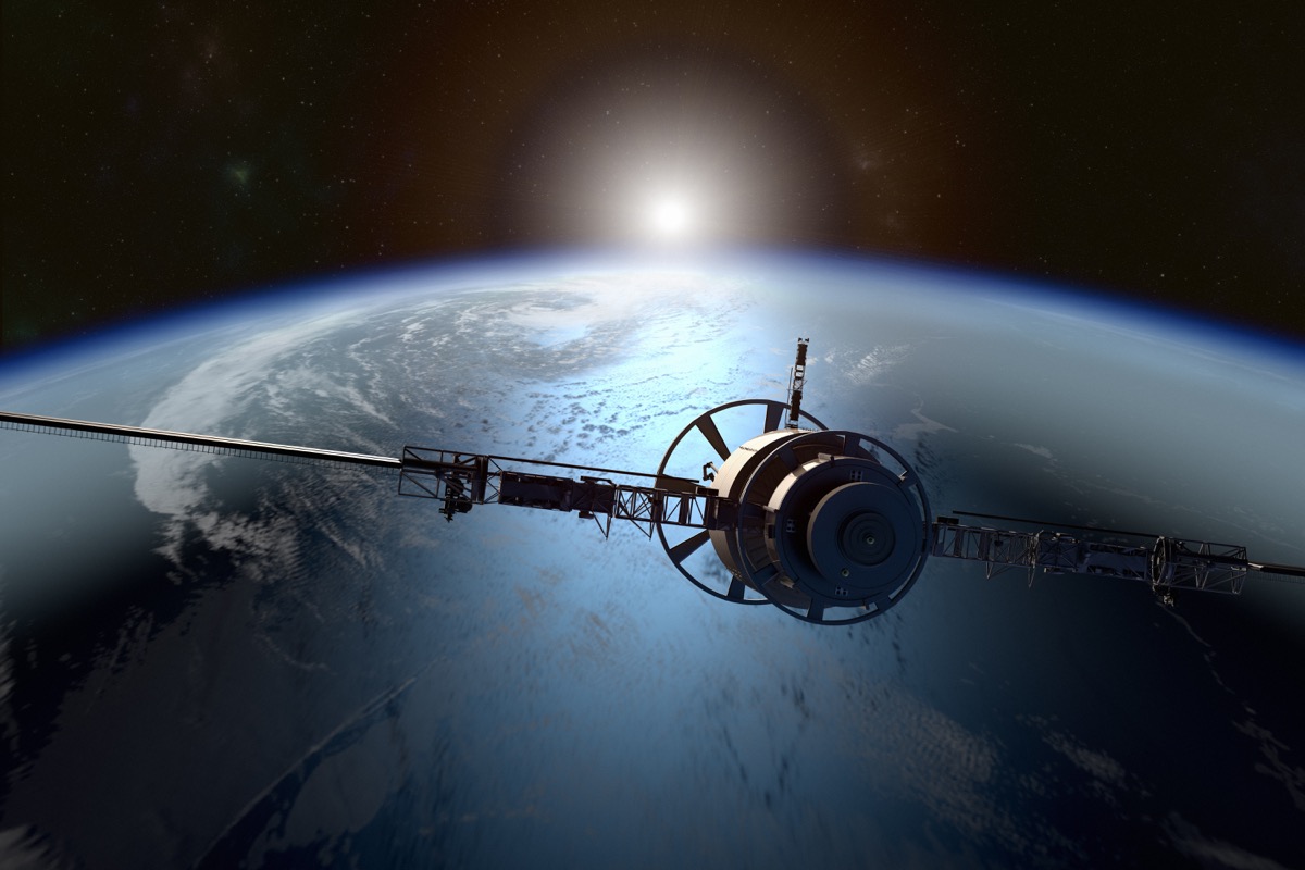
Activity Summary
The student configures a weather satellite in the Orbits and Gravitation simulation, placed at 42,164 km from Earth's centre (36,000 km altitude). The student picks the initial speed that yields a perfectly circular orbit (≈ 3.07 km/s) and observes that at this altitude the orbital period is exactly 24 hours: this is the geostationary orbit used by Meteosat, GOES and Himawari to continuously monitor a single region of the globe. The student then varies the speed to explore the regimes of falling, elliptical orbit and escape, and understands why this unique altitude is crucial for weather and climate monitoring.
Introduction
This activity studies the geostationary orbit used by weather satellites with the FizziQ Web Orbits and Gravitation simulation. The measured quantities are the circular speed and the orbital period at 36,000 km altitude. Trajectories result from Newton's universal law of gravitation applied to the Earth-satellite system.
Learning Objectives
- Identify the circular speed that gives a stable orbit and measure the corresponding period (≈ 24 hours)
- Understand why the geostationary orbit is crucial for continuous weather and climate monitoring
- Identify orbital regimes by initial speed (fall, ellipse, circle, escape)
- Connect Meteosat or GOES orbits to climate change monitoring
Scientific Concepts
Instruments and sensors
Scientific instruments
- FizziQ Web simulation (Orbits and Gravitation)
FizziQ Features
- FizziQ experiment notebook — used to record the 3-column table (initial speed, orbit type, consequence for the weather mission) and the v_esc/v_c ratio calculation.
Required Materials
- - Computer, tablet or smartphone with FizziQ Web - FizziQ experiment notebook - Note: the protocol remains adaptable to any comparable orbital-simulation tool.
Experimental Protocol
Open the Orbits and Gravitation simulation in FizziQ Web (Experiment → Simulations → Orbits and gravitation).
Set the distance scale to 200 km/pixel to see the orbit clearly, and the time scale to 10 minutes per frame to observe several revolutions quickly.
Keep body 1 as Earth (mass 1 M⊕, speed 0). Select body 2, choose "Space probe" on the mass slider (~1000 kg) and set the initial angle to -90°.
Drag the satellite to about 42,200 km from Earth's centre — use the "distances" panel in the upper right. This altitude (36,000 km above the surface) is that of geostationary weather satellites like Meteosat.
Set the initial speed to 3.07 km/s. Click the body 1 centering button to lock the view on Earth.
Click the red REC button to start recording. Observe the trajectory: the satellite traces a stable circular orbit around Earth.
Measure the period T on the chronometer in the upper-left corner: duration of one full revolution. Find T ≈ 1 day (precisely 23 h 56 min). This is the period of a geostationary orbit.
Compare T to the duration of one Earth day: since Earth also rotates on itself in 24 h, the satellite stays constantly above the same point on the ground. This is what enables Meteosat to continuously monitor Europe and Africa.
Test 2 — Speed too low: stop, set v = 1 km/s and restart. Observe that the satellite falls to Earth (collision). Without enough speed, it cannot stay in orbit and the monitoring mission fails.
Test 3 — Inner ellipse: set v = 2 km/s. Observe an elliptical orbit elongated towards Earth, the starting point becoming the apogee. Altitude varies strongly and the satellite is no longer geostationary.
Test 4 — Wider ellipses: try v = 3.5 km/s then v = 4 km/s. Observe ever-larger elliptical orbits; at 4 km/s, the satellite moves very far away before returning.
Test 5 — Escape velocity: set v = 4.5 km/s. Observe that the satellite no longer returns: it escapes on an open trajectory. Escape velocity at this altitude is about 4.35 km/s.
Fill in a 3-column table: Initial speed (km/s), Type of orbit observed, Consequence for the weather mission. Conclude that only the circular speed of 3.07 km/s allows continuous monitoring of a region.
Compute the v_esc / v_c ratio by taking 4.35 ÷ 3.07. Find a value close to 1.41 (i.e. √2), as at any altitude — this is a universal regularity of orbits.
Expected Results
At a distance of 42,164 km from Earth's centre, a speed of 3.07 km/s gives a nearly perfectly circular orbit with a period close to 24 hours, corresponding to a geostationary orbit. At 1 km/s, the satellite falls onto Earth (collision after a few simulated hours). At 2 km/s, it traces an inner ellipse, without impact but with strongly varying altitude. At 3.5 and 4 km/s, the orbit becomes elliptical outward, with an apogee moving clearly away from the geostationary trajectory. At 4.5 km/s, the satellite escapes on an open trajectory (escape velocity at this altitude is about 4.35 km/s). The v_esc / v_c ratio is about 1.41 (= √2), as at any altitude. Numerical deviations remain at a few percent due to symplectic Euler integration. This result illustrates why only precise circular orbits at 36,000 km altitude are suitable for geostationary weather satellites like Meteosat or GOES.
Scientific Questions
- Why does a geostationary satellite appear stationary in the sky as seen from the ground, even though it actually flies at 3 km/s?
- What would happen if the weather satellite orbited at 800 km altitude (low orbit, like Sentinel) instead of 36,000 km?
- Why are several geostationary satellites needed (Meteosat, GOES, Himawari) to cover the entire globe?
- How does data from these satellites accumulated over decades make it possible to evidence climate change?
Scientific Background
**Weather satellites** are observatories placed in orbit around Earth to permanently monitor the atmosphere, clouds, oceans and continental surfaces. Their data feeds daily weather bulletins and tracks climate evolution over decades.
Many of these satellites occupy a **geostationary orbit**: they orbit Earth at exactly the same angular speed as Earth rotates on itself. Seen from the ground, they appear **stationary in the sky**: a fixed antenna can therefore be aimed at them and receive their images continuously.
For an orbit to be geostationary, its **period must equal 24 hours** and the satellite must orbit in the same direction as Earth's rotation, in the equatorial plane. These conditions impose a unique altitude: about **36,000 km** above Earth's surface, or r = 42,164 km from Earth's centre.
At this altitude, the **circular speed** is about **3.07 km/s**. This is the exact speed that balances Earth's gravitational attraction on a perfectly circular trajectory.
If the speed is **lower**, the satellite descends towards Earth — either on an elliptical orbit, or in a fall down to collision. If it is **higher** but below a threshold, it traces a wider ellipse and is no longer at constant altitude: it loses its geostationary usefulness.
Above the **escape velocity** v_esc ≈ **4.35 km/s** at this altitude, the satellite escapes Earth's attraction permanently. The v_esc / v_c ratio always stays close to **1.41 (= √2)** at any altitude.
This precise orbital physics is essential for **climate monitoring**. The Meteosat (Europe-Africa), GOES (Americas) and Himawari (Asia-Pacific) satellites together cover almost the entire globe. They permanently provide images of clouds, aerosols, snow cover and ocean temperature — data essential for understanding **climate change** and the greenhouse effect.
Extensions
- Experimentally find the exact distance that gives T = 24 h while keeping the circular speed at each trial (verifying Kepler's third law)
- Reproduce the Meteosat / GOES / Himawari constellation: three satellites at 42,164 km separated by 120° around Earth, forming a geostationary trio covering the globe
- Add the Moon (at 384,400 km, speed 1.022 km/s, mass 0.012 M⊕) to the system and observe whether it perturbs the weather satellite's orbit
- Compare escape velocity from geostationary orbit (4.35 km/s) with that from Earth's surface (11.2 km/s) and explain why a satellite can "break free" more easily
Frequently Asked Questions
Why does a geostationary satellite appear stationary in the sky?
Because it orbits Earth at exactly the same angular speed as Earth's rotation (one turn in 24 h, in the same direction). Seen from the ground, it always keeps the same position in the sky, even though it actually moves at 3 km/s.
The simulation shows Earth as fixed — how can I picture Earth's rotation?
The simulation represents Earth as motionless. To visualize the geostationary nature, you must imagine Earth rotating on its axis in 24 h in the same direction as the satellite, which makes their relative positions constant.
Are there other non-geostationary weather satellites?
Yes, many. Low-orbit satellites (Sentinel, NOAA, MetOp) orbit at 800 km altitude in about 100 minutes. They give more detailed images but only fly over a given region a few times per day.
Why talk about climate monitoring and not just weather?
Weather concerns short-term forecasts (a few days). Data accumulated over decades by the same satellites allows long-term climate trends to be detected: global warming, ice melt, changes in cloud cover, sea level rise.
How does the satellite stay exactly at 36,000 km altitude without falling or escaping?
Earth's gravity pulls it towards Earth, and its 3.07 km/s speed perpendicular to this attraction keeps it on a circular trajectory. If the speed changes slightly, the orbit becomes elliptical and altitude varies. Space agencies regularly correct the trajectory with small thrusters.
Detailed Description
The student configures a weather satellite in the Orbits and Gravitation simulation, placed at 42,164 km from Earth's centre (36,000 km altitude). The student picks the initial speed that yields a perfectly circular orbit (≈ 3.07 km/s) and observes that at this altitude the orbital period is exactly 24 hours: this is the geostationary orbit used by Meteosat, GOES and Himawari to continuously monitor a single region of the globe. The student then varies the speed to explore the regimes of falling, elliptical orbit and escape, and understands why this unique altitude is crucial for weather and climate monitoring. FizziQ Web provides this orbital simulation directly in the browser, with a built-in distance readout, chronometer and REC recording tool, while the FizziQ experiment notebook lets students log the speed / orbit-type / consequence table used in the activity.
Ready to start?
Download FizziQ and try this activity with your students.