
Seven experiments to measure the speed of sound in the air
📘 The microphone is one of the phone sensors we use most in class. It serves for experiments on frequencies and on the shape of sound signals, but also for measuring the speed of sound. More on this sensor in our guide Smartphone Sensors: The Complete Guide.
- Christophe Chazot
- Apr 28
- 9 min read
Calculating the speed of sound becomes a simple and engaging task with the use of a smartphone, transforming this commonly abstract concept into a tangible learning experience. For students, this exercise is particularly gratifying as it demystifies the complexities of sound waves, allowing them to explore its various physical properties through a device that’s a familiar staple in their everyday lives. In this article, we introduce seven experiments, each utilizing a smartphone and the FizziQ app, to determine the speed of sound, making science interactive and accessible.
In short. At 20 °C, the speed of sound in air is about 343 m/s. That is “slow” enough for a smartphone to measure it with reasonable precision: done carefully, the experiments below give the result to within about 5 %, which is quite good considering that sound travels 10 meters in about 30 ms! Students can measure it through three different physical principles: the time a sound takes to travel a known distance, the resonance of an air column, and the interference of two sound waves. This guide describes seven classroom experiments that need between one and three phones and no laboratory equipment.
Contents
Sound waves and their propagation - Methods for measuring the speed of sound - Measurement by time of flight - Measurement by wavelength - Measurement by resonance frequency - Conclusion
Sound waves and their propagation
A sound wave is a mechanical vibration that propagates through a medium, such as air or a liquid. The speed of sound is the speed at which this wave propagates in this medium, it depends on the temperature, the pressure and the density of the medium through which it propagates.
In air, if we assimilate it to a perfect diatomic gas, we can calculate the speed of sound by the equation: c = sqrt(γ*RT/Ma), c, the speed of sound, γ, the ratio of heat capacities at constant pressure and volume. γ= 7/5 for air, R, the ideal gas constant, T, the absolute temperature of the medium, Ma, the molar mass of air: Ma = 29g/mol.
Using the previous formula we can calculate the theoretical speed of sound at the usual conditions of temperature and pressure: c = 343 m/s for a temperature of 20 degrees, or approximately 767 miles per hour. In water, sound travels more than 4 times faster than in air, i.e. at about 1,482 meters per second, and in some metals like soft iron, it travels significantly faster at close to 6,000 m/s (13,333 miles per hour).
How to measure the speed of sound with a smartphone?
There are many different ways to measure the speed of sound using a smartphone or a tablet. These methods fall into three broad categories, which, interestingly, use different physical characteristics of sound waves :
- Estimating the time of flight (ToF)
- Measuring the sound frequency using an Helmholtz resonator
- Measuring the wavelength at a given frequency
Here are the seven experiments side by side. The accuracies are those we obtain in class, not the best possible ones.
| # | Experiment | Principle | Phones | Equipment | Typical accuracy | Level | Time |
|---|---|---|---|---|---|---|---|
| 1 | Acoustic stopwatch, two claps | Time of flight | 2 | Tape measure, 5 to 20 m of space | 3 to 8 % at 10 m or more | Middle and high school | 30 min |
| 2 | Synchronized stopwatches | Time of flight | 2 | Same | 5 to 10 % | Middle and high school | 30 min |
| 3 | Test tube and water | Resonance | 1 | Graduated cylinder, water, ruler | About 1 % with linear regression | High school | 35 min |
| 4 | Blowing across a bottle | Resonance | 1 | An empty bottle, ruler | 10 to 15 % | High school | 20 min |
| 5 | The pop of a cork | Resonance | 1 | A bottle to open | 10 to 15 % | High school | 20 min |
| 6 | Tube and white noise | Resonance | 2 | Cardboard tube, ruler | 5 to 10 % | High school | 30 min |
| 7 | Interference of two sources | Wavelength | 2 or 3 | Tape measure, a quiet room | About 10 % | High school | 45 min |
These are the methods that have been used by generations of scientists to determine the speed of sound:
➡️ Marin Mersenne, the first, evaluated in 1635 the speed of sound in air at 448 m/s by the propagation time method. Value further refined by the scientists Viviani and Borelli in 1656 with a value of 344 m/s.
➡️ Isaac Newton took a different approach through an analytical method by determining it from the resonant frequencies of sound waves in a U-tube and details his method in the first edition ofIt begins (1687).
➡️ Over the centuries, as estimations were more accurate, one uncertainty remained: could humans go faster than the speed of sound? This question will be resolved in 1947 when American aviator Chuck Yeager reached Mach 1 aboard the X-1 aircraft. Once again, the human had crossed an impassable barrier.
Now, the iconic measurement of the speed of sound is readily accessible to anyone. You can delve into these experiments using one or more smartphones, with no need for specialized equipment. Embark on a journey of discovery right at your fingertips, grab your cellphones and let’s dive into this exciting venture!
Measuring the Time of Flight (ToF)
Like any speed calculation, the objective here is to determine the time it takes for a sound wave to travel a certain distance. The speed of sound being high, the measurement of time requires a specific equipment: an acoustic stopwatch.
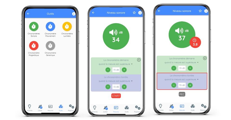
An acoustic stopwatch measures the time difference between two sounds which sound level exceeds a certain threshold. This device cannot be found on a lab bench but many smartphone applications exist that offer this functionality. In FizziQ, you will find the acoustic stopwatch in the Tools menu. You can also build your own acoustic stopwatch using triggers.
If you have never used the acoustic stopwatch before, the activity Reflexes is a good warm-up: it compares a manual stopwatch with the FizziQ acoustic stopwatch and helps students get a feel for the precision of the tool before tackling the speed-of-sound measurement.
 Measure of the speed of sound using Time of Flight (ToF)**The traditional protocol for measuring the speed of sound **with an acoustic stopwatch is as follows: two smartphones are separated by a certain distance (at least 5 meters), and an operator is placed near each telephone. The operators clap their hands one after the other. The first clap starts both stopwatch and the seconds stops them. Students then check that the time difference dt between the two stopwatches is dt = 2*d/c, where d is the distance between the smartphones, c the speed of sound. This experiment allows an accuracy between 3 and 8 % from 10 m upwards, and can be improved by performing several measurements. An opportunity to do a bit of statistics as well !
Experiment 1 at a glance. What you need: two phones with an acoustic stopwatch, a tape measure, 5 to 20 m of open space. How it works: the first clap starts both stopwatches, the second stops them; the sound of each clap reaches the far phone later than the near one. Formula: dt = 2·d/c. Expected result: at 10 m, dt ≈ 58 ms. Accuracy: 3 to 8 % from 10 m upwards, better with several runs. Common errors: distance too short (at 5 m, dt is only 15 ms, close to the trigger precision of ±1 to 2 ms), a trigger level that fires on footsteps, wind along the line of the phones.
The protocol works well, but younger students find it often difficult to understand the offset formula calculation which is not very intuitive. We prefer a variation of this protocol developed by Aline Chaillou of the La main à la pâte Foundation.
In this second protocol, **we start by synchronizing the chronometers **by putting them side by side and trigger the sound chronometers by clapping our hands. Then, we move one of the two smartphone by a certain distance d without making noise. An operator located near this second laptop then stops the two stopwatches by clapping his hands. The calculation of the shift is then very intuitive for the students because they have immediately put in relation the difference in distance which creates the phase shift with the displacement of one of the two smartphones.
The time difference dt is equal to: dt = d/c.
This simplicity has a price. In the first protocol each clap is heard by both phones, so the measured delay corresponds to the sound covering the distance d twice: that is what the factor 2 means. For the same trigger error (±1 to 2 ms), experiment 1 is therefore about twice as precise as this one, 3 to 8 % against 5 to 10 %. The synchronized variant is easier to explain but a little less accurate; make up for it with a longer distance.
This second protocol also makes it possible to introduce the notion of clock synchronization. It is the same concept of synchronization that was used in the famous Hafele-Keating experiment in 1971 to prove relativity. Be mindful to calibrate the trigger level of the sound stopwatch so that it does not trigger when you move one of the two smartphones.
The full step-by-step protocol — including the synchronization variant and the data analysis — is available in the activity Speed of sound.
Experiment 2 at a glance. What you need: the same two phones and tape measure. How it works: the stopwatches are started side by side, one phone is carried away quietly, a single clap next to it stops both. Formula: dt = d/c. Expected result: 29 ms at 10 m, 58 ms at 20 m. Accuracy: 5 to 10 %, since the measured delay is half that of experiment 1; the standard deviation over repeated runs drops quickly with distance. Common errors: the stopwatch of the moving phone triggered during the walk, a distance measured to the wrong point of the phone.
Measuring the speed of sound with Helmholtz resonators
The second method of** calculating the speed of sound is based on the principle of acoustic resonance,** which is a phenomenon in which an acoustic system amplifies sound waves whose frequency corresponds to one of its own frequencies of vibration. The resonance frequencies of certain cavities like a cylinders or a bottles are easy to determine by calculus. This frequency depends on the speed of sound and the shape of the object. By measuring the resonance frequency we can infer the speed of sound.
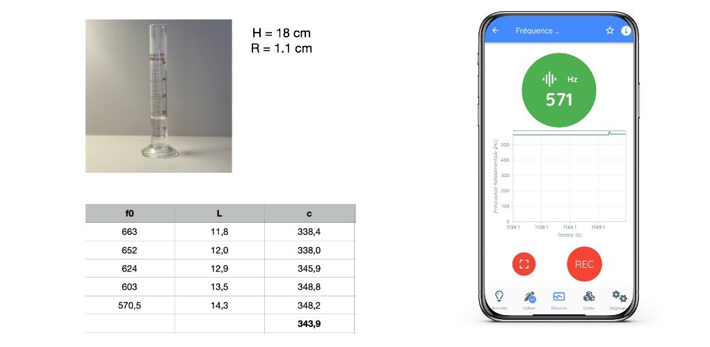
A very simple first protocol consists of blowing on the edge of a graduated test tube. This emits a sound for which we can measure the fundamental frequency using FizziQ. For a closed tube, the fundamental resonance frequency is: f₀ = c/(4·L + 1.6·D), where L is the length of the tube, D is the diameter of the tube.
To make more precise measurements, we can measure the frequency for different heights of water in the test piece, and by doing a linear regression of the results, we can accurately determine the speed of sound to less than one percent. This precise version of the protocol — with linear regression on multiple water heights — is detailed in the activity Helmholtz.
Experiment 3 at a glance. What you need: one phone with a frequency meter or spectrum analyzer, a graduated cylinder, water, a ruler. How it works: blowing across the rim excites the fundamental of the air column; adding water shortens the column and raises the note. Formula: f₀ = c/(4·L + 1.6·D). Expected result: from about 200 to 400 Hz with the cylinder empty up to 800 to 2000 Hz with 2 or 3 cm of air left; f plotted against 1/L is a straight line whose slope gives c. Accuracy: around 1 % with the regression, 5 to 10 % from a single reading. Common errors: forgetting the end correction (c comes out too high by 5 to 10 %), an unsteady note (readings scatter by ±5 to 10 Hz).
 Measuring the speed of sound using Helmholtz resonatorIf you are a Bordeaux lover and have an empty bottle, you can use a bottle from this region whose volumetric characteristics are immutable. Ulysse Delabre in this video details the calculations for measuring the resonance frequency when blowing into the bottle.
A complete walk-through of this experiment, with frequency measurement of the “pop” and calculation of the speed of sound from the bottle’s geometry, is provided in the activity The sound of a bottle.
Experiment 4 at a glance. What you need: one phone, an empty bottle, a ruler. How it works: the bottle is a Helmholtz resonator, the air in the neck oscillates on the cushion of air in the body. Formula: f₀ = (c/2π)·√(A/(V·L’)), with A the neck cross-section, V the volume of air and L’ the neck length plus its end correction (about 0.6·D). Expected result: 300 to 600 Hz depending on the bottle, 400 to 500 Hz for a standard 75 cl wine bottle. Accuracy: 10 to 15 %. Common errors: the internal volume and the neck dimensions, which are hard to measure well and dominate the uncertainty.
What if the bottle is unopened? It is still possible to carry out the experiment and, paradoxically, in an even simpler way: by uncorking it! When the cork is removed, a “pop” is heard which is due to the resonance of the air in the part between the liquid and the top of the bottle. If we measure the frequency of pop with the frequency meter, we can use the previous formula of the resonant frequency of a tube to deduce the speed of sound.
Experiment 5 at a glance. What you need: one phone with the frequency meter, a bottle to open. How it works: the pop is the air in the neck resonating for a few hundredths of a second. Formula: same as experiment 4, with V the volume of air between the liquid and the cork. Expected result: a short peak between 300 and 600 Hz. Accuracy: 10 to 15 %. Common errors: a pop too short for the meter to lock on (record it and read the spectrum instead), a level of liquid not measured.
A last protocol which always surprises students uses the fact that if several frequencies are emitted simultaneously in a cavity, the harmonics of the resonant frequency of the cavity will be amplified compared to the other emitted frequencies. If we measure the spectrum of a white noise emitted in this cavity, the harmonic frequencies of the resonant frequency are highlighted compared to the others. It is recalled that white noise is a random succession of sound emitted in all frequencies. White noise sounds can be found in FizziQ’s sound library. Students unfamiliar with white noise can first explore its frequency content with the activity White noise, which uses the FizziQ spectrum analyzer to show that white noise contains all frequencies at roughly equal intensity.
So let’s take a tube open at both ends, such as a paper towel roll or a vacuum cleaner hose. At one end of the tube, we will emit a white noise that can be generated with the FizziQ sound library or by using the sound of a video emitting white or pink noise. At the other end of the tube, we measure the frequency spectrum. Measuring the white noise spectrum through a tube will show peaks for the fundamental frequency and its harmonics. We deduce the resonance frequency then the speed of sound by the formula of the resonance frequency of an open tube : f₀ = c/(2·L + 1.6·D)
The full protocol — with white-noise emission, spectrum analysis at the other end of the tube, and identification of the resonance peaks — is described in the activity Tube effect.
Experiment 6 at a glance. What you need: two phones (one plays the noise, one analyzes the spectrum), a cardboard tube, a ruler. How it works: the tube amplifies the frequencies that fit its length; the peaks of the spectrum are the fundamental and its harmonics. Formula: f₀ = c/(2·L + 1.6·D), harmonics at 2f₀, 3f₀… Expected result: for a paper towel roll 30 cm long and 4 cm wide, a fundamental near 540 Hz, then peaks near 1090, 1630 and 2170 Hz. Accuracy: 5 to 10 %, better if you use several tube lengths and take the slope. Common errors: reading a harmonic as the fundamental, forgetting the end correction (8 to 15 % too high).
Better results are often obtained with pink noise, which is similar to white noise, but with a reduced loudness for high-pitched sounds. The use of pink noise makes it possible to reinforce the intensity of the fundamental resonant frequency compared to its higher harmonics. Examples of of pink noise can be found on internet.
Finally, one can make different measurements with different sizes of the tube, and deduce c by measuring the slope on the graph.
Measuring the speed of sound with waves interferences
This third type of protocol is based on measuring the wavelength of a pure sound of known frequency. We deduce the speed by the relation: c = l.f, with l the wavelength and f the frequency.
This method is the one usually used in the school labs. It uses **a sound source and two microphones placed at a certain distance from this source and connected to an oscilloscope with a dual input. **By moving the two microphones relative to each other, the operator finds the distance for which the two waves are in phase, which is the wavelength.
With smartphones, this protocol is not possible because they do not have dual sound inputs… However with a little imagination we can find other ways!
The first protocol that we propose consists in using two smartphones that emit the same pure sound, for example at a frequency of 680 hertz. By placing the smartphones at a certain distance, we will calculate the places along the two smartphones axis where waves add up and places where they cancel.
With FizziQ one can use the sound at 680 hertz from the sound library. Two smartphones are placed about 3 meters from each other. A third smartphone is used to measure the sound intensity (oscillogram instrument on FizziQ) along the axis of the two smartphones. The interference of the two waves creates zones of very high intensities, the antinodes, and other very weak ones, the nodes. The distance between the nodes (about 50 cm) is equal to the wavelength of the sound wave for the frequency 680 hertz. By measuring the difference between the nodes (or the bellies), we calculate the speed of sound.
This three-smartphone interference experiment is fully detailed in the activity A bubble without noise, which guides students through locating the nodes and antinodes and computing the wavelength — and from it, the speed of sound.
The experiment can also be carried out with only two mobile phones. One of the two smartphones then serves as a transmitter, and also as a tool for measuring the sound volume. A second mobile that emits a pure sound of the same frequency is approached to the first, and the distance between the knot and the belly is noted by measuring the sound volume on the first smartphone, identified by the variations in intensity. To carry out this experiment with FizziQ, we prefer to use the sound intensity measured with the Oscilloscope instrument and which is more precise than the sound volume in decibels.
Finally, if you only have a smartphone, it is also possible to carry out this experiment by placing a reflective surface in place of the second smartphone from the previous experiment. The precision is further reduced but the calculation is nevertheless possible!
Experiment 7 at a glance. What you need: two phones playing the same pure tone and a third one measuring the level, or two phones only, in a room with few echoes. How it works: where the two waves arrive in phase the sound is loud, where they arrive in opposition it almost vanishes. Formula: c = λ·f, with λ measured from the pattern. Expected result: at 680 Hz, successive minima about 25 cm apart, that is half a wavelength; at 440 Hz, about 39 cm. Accuracy: about 10 %. Common errors: reflections from walls and furniture that blur the minima, speakers of unequal loudness, a level meter moved too fast.
These different experiments make it possible to calculate the speed of sound with an accuracy of about 10%.
Which method should I use?
It depends on what you have in the cupboard and on what you want the class to understand.
- With one phone only: the test tube (experiment 3) or a bottle (4 and 5). No partner needed, and the regression version of the test tube is the most accurate of the seven.
- For middle school: the synchronized stopwatches (experiment 2). Students see the delay appear as they walk the phone away; the formula dt = d/c needs no explaining.
- For the most accurate result: the test tube with several water heights and a linear regression (experiment 3). We regularly get within 1 % of the tabulated value.
- To show what resonance is: the tube and white noise (experiment 6). The spectrum on the screen, with its evenly spaced peaks, is the standing wave made visible.
- To show interference: the two sources (experiment 7). Walking through the loud and silent zones with the level meter is something students remember.
- Outdoors, with a large group: the acoustic stopwatches (1 and 2). Give each pair of students a distance and compare the results on the board.
- Indoors, in a small room: prefer resonance (3 to 6). Echoes spoil the stopwatch and interference measurements.
What to expect, and where the errors come from
Whatever the method, a careful class ends up between 330 and 360 m/s. The tabulated value is 343 m/s at 20 °C, so a result of 335 m/s in a cold corridor at 12 °C is not a mistake: the speed of sound gains about 0.6 m/s per degree, and 338 m/s is what the formula gives at that temperature. Ask students to note the temperature before they start.
With the stopwatches, the limiting factor is the trigger, which fires with a precision of about ±1 to 2 ms. Over 5 m the delay to measure is only 15 ms, and the standard deviation over ten runs is typically 5 to 15 %. Over 20 m the delay is 58 ms and the spread falls to 5 to 10 %. With the two claps of experiment 1 the measured delay doubles (117 ms at 20 m) for the same trigger error, and the spread comes down to 3 to 8 %. Distance is the cheapest way to buy accuracy.
With resonance, the trap is the end correction. The air column vibrates a little beyond the opening, so the effective length is longer than the tube: 0.6·D per open end, hence the 1.6·D and 4·L terms in the formulas above. Leave it out and the speed of sound comes out too high by 5 to 15 %, which is exactly the systematic error students find when they compare with the tabulated value. Finding that error themselves is worth more than the corrected number.
With interference, the pattern is never as clean as the drawing. Minima are shallow because of reflections, and readings scatter by ±2 to 3 dB. Measuring several fringes and dividing is what brings the result back to 10 %.
The tools, in 2026
All seven experiments were designed for FizziQ, which today provides the acoustic stopwatch, the frequency meter, a real-time spectrum analyzer, a sound generator with pure tones and white and pink noise, and the notebook in which the measurements, photos and calculations end up. FizziQ Web runs the same sound instruments on a computer, which is convenient for the regression of experiment 3 or for projecting a spectrum to the whole class. Any other app with an acoustic stopwatch and a spectrum analyzer will do; the physics does not change.
To conclude
We have identified a number of different ways to estimate the speed of sound. These experiments can be classified into three categories that relate to different physical properties of sound waves. All of these experiments can be done with FizziQ, or with other mobile or tablet apps, depending on your preference. The smartphone is one of the best tools available for measuring the speed of sound, offering multiple ways to approach the same problem, and easily accessible to students. Happy experimenting!
Frequently asked questions
What is the speed of sound at 20 °C? About 343 m/s in dry air, or 1,235 km/h. It does not depend on the pressure at a given temperature, but it does depend on the temperature: about 331 m/s at 0 °C, 343 m/s at 20 °C, 349 m/s at 30 °C.
Can I measure the speed of sound with one phone? Yes, with resonance. A graduated cylinder and some water (experiment 3) or a bottle (experiments 4 and 5) only need one phone with a frequency meter. The test tube with a regression is even the most accurate method of the seven.
Why do I need two smartphones for the time-of-flight method? Because sound covers 10 m in 29 ms, far too fast for one person with one stopwatch. Two acoustic stopwatches, one at each end, record the arrival of the same clap at two places; the difference between them is the travel time.
Does the frequency change the speed of sound? No. In air, at audible frequencies, a 100 Hz sound and a 5,000 Hz sound travel at the same speed. Students can check it with the interference experiment at two frequencies: the fringe spacing changes, the calculated speed does not.
How does the temperature affect the result? The speed of sound rises by about 0.6 m/s per degree Celsius. A measurement made outside at 10 °C should give about 337 m/s, not 343. Write down the temperature and compare with the value expected at that temperature, not with the textbook figure.
Which method is the most accurate? The test tube with several water heights and a linear regression, within about 1 %. Then the two-clap acoustic stopwatch (experiment 1) at 20 m or more, within 3 to 8 %; the synchronized variant is easier to explain but a little less accurate, 5 to 10 %. Bottles and interference are closer to 10 %.
Can I do these experiments indoors? Resonance experiments (3 to 6) work anywhere. The stopwatches and the interference experiment suffer from echoes: a gym or a corridor gives blurred minima and false triggers. Take them outside, or into the largest and most furnished room available.
What is the end correction, and can I ignore it? The air in a tube vibrates slightly beyond the opening, so the tube behaves as if it were about 0.6 times its diameter longer at each open end. Ignoring it makes the speed of sound come out 5 to 15 % too high. Keeping it in the formula is what brings the test tube down to 1 %.
Further reading: this article is part of our complete guide to measuring and analyzing sound with a smartphone or computer.