
1. Introduction
1.1 What is FizziQ Web?
FizziQ Web is a free web application that supports students throughout their scientific and experimental process. From data capture to communicating results, FizziQ Web provides all the tools needed to run a complete experimentation session on a computer.
1.2 The three pillars of FizziQ Web
FizziQ Web is organized around three main features that correspond to the three stages of the scientific process:
1. Experiment
Capture data
2. Analyze
Organize and understand
3. Share
Communicate your results
Experiment: capturing data
FizziQ Web offers five data sources, all compatible with one another:
- Audio analysis: recording and analyzing sound through the computer's microphone (sound level, frequency, spectrum, spectrogram)
- Kinematic analysis: tracking videos and chronophotographs to study motion (positions, velocities, accelerations)
- External sensors: connection to FizziQ Connect or microcontrollers (Arduino, micro:bit) via Bluetooth or USB
- Manual entry: creating data tables filled in by the student
- Simulations: virtual experiments (pendulum, spring, ballistics, circuits, waves, ideal gas...) generating usable data
Analyze: organizing and understanding data
All captured data arrives in the experiment notebook as observation cards. The student can:
- Organize their data in tables
- Add columns and create calculated quantities (formulas)
- Define the units of each quantity
- Create graphs with different scales
- Perform modeling and curve fitting
Share: communicating your results
Once the analysis is complete, the student can create a final report that summarizes their research:
- Writing explanatory text
- Inserting photos and diagrams
- Integrating tables and graphs from the experiment notebook
- Adding mathematical formulas (LaTeX syntax)
- Exporting to PDF, Word, or image
1.3 Detailed features
Audio analysis
Waveform, spectrum, spectrogram
Video analysis
Tracking, kinematics, trajectories
Chronophotographs
Import and motion analysis
Simulations
Pendulum, spring, waves, gas...
FizziQ Connect
External Bluetooth/USB sensors
Data tables
Data, formulas, graphs
Report editor
Reports with LaTeX formulas
Python
Built-in interpreter
1.3 Browser compatibility
| Browser | Audio | Video | Simulations | Bluetooth | USB |
|---|---|---|---|---|---|
| Chrome | Yes | Yes | Yes | Yes | Yes |
| Edge | Yes | Yes | Yes | Yes | Yes |
| Firefox | Yes | Yes | Yes | No | No |
| Safari | Yes | Yes | Yes | No | No |
1.4 Differences from FizziQ mobile
FizziQ Web complements the mobile application:
- No built-in sensors: a computer has no accelerometer or GPS (use FizziQ Connect for external sensors)
- Advanced audio analysis: high-resolution spectrogram, detailed analysis
- Complete video analysis: kinematic tracking, calculation of velocities and accelerations
- Physics simulations: pendulum, spring, ballistics, circuits, waves, ideal gas, inclined plane, centrifuge
- Larger screen: ideal for data analysis, graphs, and reports
- Document editor: scientific reports with LaTeX formulas
1.5 Privacy and free access
2. Getting started
2.1 Accessing FizziQ Web
- Open your Chrome or Edge browser
- Go to fizziqweb.web.app
- Click Experiment to access the tools
2.2 General interface
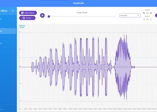
The FizziQ Web interface is organized around a left-hand side menu:
- Home: home page and quick access
- Experiment: access to the analysis and simulation modules
- Audio analysis
- Video analysis
- Chronophotographs
- External sensors (FizziQ Connect)
- Data table
- Simulations
- Analyze: data analysis tools
- Share: screen sharing and export
- Discover: educational activities and resources
- Tools: additional tools (calculator, synthesizer...)
- Settings: application settings
2.3 Your first measurement: analyzing a sound
Here is how to carry out your first audio analysis:
- Click Experiment → Audio analysis
- Click Audio Source → Sound library
- Select Tuning fork A3 (440 Hz)
- Observe the waveform and the frequency spectrum
- Use the scroll wheel or the Zoom buttons to see the details
- Click Add to notebook to export the analysis
3. Audio analysis - Experiment
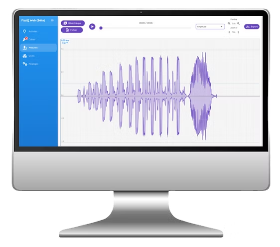
3.1 Audio sources
You can analyze sound in several ways:
- Record with the computer's microphone
- Load an audio file (WAV, MP3, OGG, FLAC, M4A)
- Built-in sound library
Sound library
The built-in library offers many educational sounds:
- 440 Hz tuning fork: pure reference tone
- Musical instruments: piano, guitar, flute, violin...
- White noise: all frequencies
- Siren: frequency variation
- Doppler effect: demonstration of the frequency shift
- Risset bells: auditory illusion of an endless rise
- Beats: interference of two nearby frequencies
3.2 Analysis modes
| Mode | Display | Use |
|---|---|---|
| Amplitude | Time-domain waveform (oscillogram) | Observe the structure of the sound, measure the period |
| Sound level (dB) | Intensity in decibels | Measure the volume, compare sources |
| Fundamental frequency | Main frequency (Hz) | Identify a note, tune an instrument |
| Spectrum | Frequencies at an instant | Analyze harmonics, timbre |
| Spectrogram | Time-frequency evolution | Complex sounds, melodies, voice, Doppler effect |
3.3 Reading the spectrogram
The spectrogram displays the evolution of the frequency spectrum over time. It is a powerful tool for analyzing complex sounds.
Color code:
- Black: silence
- Blue: low intensity
- Yellow: medium intensity
- Red: maximum intensity
Examples of spectrogram uses
- Melody: observe the successive notes
- Voice: analyze formants and harmonics
- Doppler effect: visualize the frequency shift
- Instruments: compare timbres
3.4 Measurement tools
- Interactive cursor: click on the graph to measure a precise point
- Zoom: scroll wheel or +/- buttons to enlarge
- Synchronization: audio playback synchronized with the display
- Min/max display: visualize the envelope of the signal
3.5 Exporting audio data
Depending on the analysis mode, you can export:
- Amplitude mode: Time (s), Amplitude
- Frequency mode: Time (s), Frequency (Hz)
- Spectrum mode: Frequency (Hz), Magnitude
- Spectrogram: data table or image
4. Video analysis - Experiment
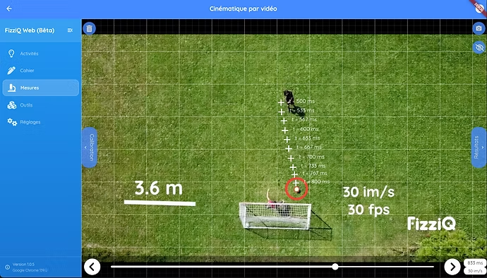
FizziQ Web includes a complete kinematic video analysis module, allowing you to study the motion of objects from videos.
4.1 Importing videos
Supported formats: MP4, WebM, MOV, AVI, and most common video formats.
- Click Experiment → Video analysis
- Click Load a video
- Select your video file
- The video appears in the tracking interface
4.2 Scale calibration
Before tracking, you must calibrate the scale to convert pixels into meters:
- Click Calibrate the scale
- Click on the two ends of a reference object (ruler, meter stick...)
- Enter the actual length of the object
- The scale is set for the entire analysis
4.3 Tracking positions
Tracking consists of recording the position of an object frame by frame:
- Select the point to track (center of the object)
- Click on the object in the first frame
- Advance to the next frame (button or arrow)
- Click on the new position of the object
- Repeat until the end of the motion
4.4 Automatically calculated quantities
From the tracked positions, FizziQ Web automatically calculates:
| Quantity | Symbol | Description |
|---|---|---|
| Position x | x(t) | Horizontal position as a function of time |
| Position y | y(t) | Vertical position as a function of time |
| Velocity vx | vx(t) | Horizontal component of the velocity |
| Velocity vy | vy(t) | Vertical component of the velocity |
| Velocity | v(t) | Magnitude of the velocity |
| Acceleration ax | ax(t) | Horizontal component of the acceleration |
| Acceleration ay | ay(t) | Vertical component of the acceleration |
| Acceleration | a(t) | Magnitude of the acceleration |
| Angle | θ(t) | Angle of rotation (for rotational motion) |
| Kinetic energy | Ec(t) | ½mv² (if the mass is defined) |
| Potential energy | Ep(t) | mgh (if the mass is defined) |
4.5 Calculation methods
FizziQ Web offers several methods to calculate derivatives (velocity, acceleration):
- Linear interpolation: simple method, suited to slow motion
- Quadratic interpolation: more accurate method, reduces noise
- Smoothing: attenuation of measurement noise
4.6 Examples of video experiments
- Free fall: verify that a = g ≈ 9.8 m/s²
- Projectile launch: study the trajectory, verify that vx = constant
- Circular motion: analyze the rotation, calculate the centripetal acceleration
- Oscillations: study a filmed pendulum or spring
- Collisions: verify the conservation of momentum
- Camera fixed on a tripod
- Uniform background contrasting with the object
- Good lighting
- Reference object visible for calibration
- High frame rate (60 fps or more for fast motion)
5. Chronophotographs - Experiment
A chronophotograph is an image showing the successive positions of a moving object, superimposed on a single image. FizziQ Web lets you analyze these images and also create them from videos.
5.1 Importing a chronophotograph
- Click Experiment → Chronophotographs
- Click Load an image
- Select your image file (PNG, JPG...)
- Calibrate the scale as for video
- Track the successive positions of the object
5.2 Creating a chronophotograph from a video
FizziQ Web can convert a video into a chronophotograph:
- Go to Tools → Video → chronophotograph converter
- Load your video
- Select the time interval between frames
- Choose the number of frames to superimpose
- Export the resulting image
5.3 Kinematic analysis
Analyzing a chronophotograph gives the same quantities as video analysis:
- Positions x(t) and y(t)
- Velocities vx(t) and vy(t)
- Accelerations ax(t) and ay(t)
- Trajectory in the (x, y) plane
5.4 Examples of chronophotographs
- Ball in free fall: increasing spacing (acceleration)
- Uniform motion: constant spacing
- Projectile: visible parabola
- Bounce: analysis of the phases before and after the impact
6. Physics simulations - Experiment
FizziQ Web offers eight interactive simulations that generate data usable in the experiment notebook. Each simulation lets you place virtual sensors and record measurements in real time.
6.1 Pendulum simulation
Objective: Study the oscillatory motion of a simple pendulum.
Parameters
| Parameter | Range | Default |
|---|---|---|
| Pendulum length | 0.2 - 5.0 m | 2.0 m |
| Initial angle | 5° - 85° | 30° |
Measurable quantities
- Tangential acceleration: at = -g sin(θ)
- Centripetal acceleration: an = L ω²
- Angle θ as a function of time
- Angular velocity ω
- Kinetic and potential energy
Usage
- Set the length and the initial angle
- Place the desired virtual sensors
- Click REC then START to record
- Click STOP to stop
- The data is automatically added to the notebook
6.2 Spring oscillator simulation
Objective: Study the oscillations of a mass-spring system.
Parameters
| Parameter | Range | Default |
|---|---|---|
| Spring stiffness (k) | 1 - 100 N/m | 20 N/m |
| Mass | 0.1 - 5.0 kg | 0.5 kg |
| Initial amplitude | 0.05 - 1.0 m | 0.3 m |
| Damping | 0 - 2.0 N.s/m | 0 |
Measurable quantities
- Position (elongation) x
- Velocity dx/dt
- Acceleration a = -(k/m)x - (b/m)v
- Kinetic energy and elastic potential energy
6.3 Ballistics simulation
Objective: Study the trajectory of a projectile.
Parameters
| Parameter | Range | Default |
|---|---|---|
| Initial velocity (v₀) | 10 - 100 m/s | 50 m/s |
| Launch angle (α) | 15° - 85° | 45° |
| Projectile mass | 0.1 - 10 kg | 1 kg |
| Air resistance | Toggleable | Disabled |
Equations (without friction)
- Horizontal position: x(t) = v₀ cos(α) t
- Vertical position: y(t) = v₀ sin(α) t - ½ g t²
- Maximum range at 45°: R = v₀² sin(2α) / g
With air resistance
Enable drag to observe:
- Reduction of the range
- Asymmetry of the trajectory
- Dependence on the mass
6.4 Electrical circuit simulation
Objective: Build and analyze electrical circuits.
Available components
- Sources: battery (DC voltage), AC generator (variable voltage)
- Elements: wires, resistors, lamps, switches, diodes
- Instruments: ammeter (in series), voltmeter (in parallel)
Building a circuit
- Click a component in the toolbar
- Move it into the work area
- Connect the terminals by dragging them
- The circuit works as soon as it is closed
6.5 Inclined plane simulation
Objective: Study uniformly accelerated rectilinear motion.
Parameters
| Parameter | Range | Default |
|---|---|---|
| Angle of inclination | 5° - 90° | 30° |
| Distance to travel | 1 - 10 m | 10 m |
| Coefficient of friction | 0 - 1 | 0 |
Physics
- Acceleration: a = g sin(θ) - μ g cos(θ)
- At 90°: motion = free fall
- Galileo's principle: slow down free fall to observe it better
6.6 Waves on a lake simulation
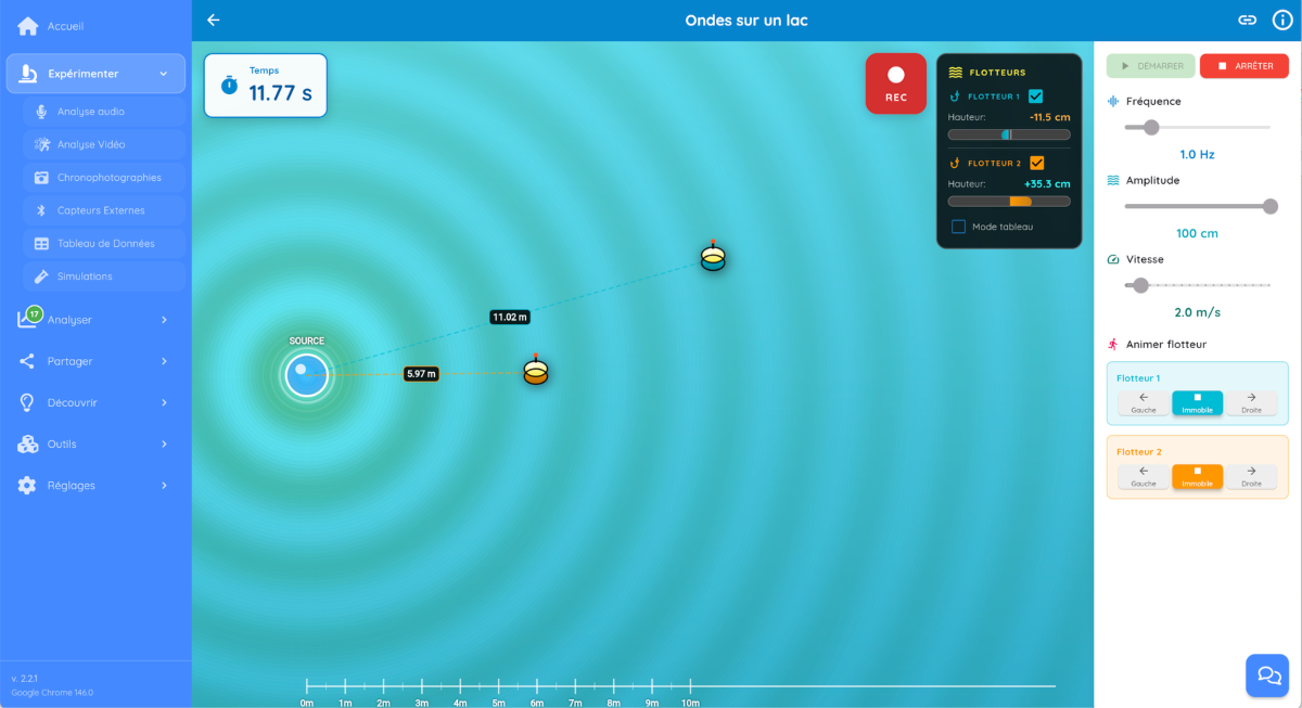
Objective: Study the propagation of waves on the surface of water.
Parameters
| Parameter | Range | Default |
|---|---|---|
| Frequency | 0.1 - 5 Hz | 1 Hz |
| Amplitude | 1 - 100 cm | 100 cm |
| Propagation speed | 0.5 - 5 m/s | 2 m/s |
Features
- Source: generates the waves
- Floats: measure the height of the water at their position
- Table mode: displays the float data
- Float animation: individual control of the motion
Observable phenomena
- Circular propagation of waves
- Relationship λ = v / f (wavelength = speed / frequency)
- Phase shift between two points
- Interference (with several sources)
6.7 Ideal gas simulation
Objective: Study the laws of ideal gases.
Parameters
| Parameter | Description |
|---|---|
| Volume | Volume of the container (adjustable with a piston) |
| Temperature | Temperature of the gas |
| Number of particles | Amount of substance |
Verifiable laws
- Boyle-Mariotte's law: PV = constant (at constant T)
- Gay-Lussac's law: P/T = constant (at constant V)
- Charles's law: V/T = constant (at constant P)
- Equation of state: PV = nRT
6.8 Centrifuge simulation
Objective: Study circular motion and centrifugal forces.
Measurable quantities
- Angular velocity ω
- Centripetal acceleration ac = ω²R
- Apparent centrifugal force F = mω²R
- Rotation period T = 2π/ω
7. External sensors - Experiment
FizziQ Web lets you connect external sensors to take real physical measurements. Two options are available to you:
FizziQ Connect
Plug-and-play box, instant connection
For microcontrollers (Arduino, micro:bit, ESP32...), see the Appendix: Connecting microcontrollers, which details the data format and code examples.
7.1 FizziQ Connect: overview
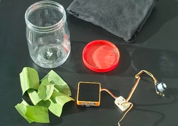
FizziQ Connect is a data acquisition box (computer-assisted experimentation) that lets you connect external sensors to FizziQ Web. Based on the ESP32 microcontroller, it uses standard Grove sensors.
7.2 Compatible sensors
| Type | Sensors |
|---|---|
| Temperature | Temperature probe, thermocouple |
| Pressure | Atmospheric pressure sensor, manometer |
| Light | Light meter, UV sensor |
| Air quality | CO2 sensor, particle sensor |
| Distance | Ultrasonic sensor, infrared sensor |
| Electricity | Voltage probe, current probe |
| Analog | Any analog sensor (including those built by students) |
7.3 Bluetooth connection
Advantages: wireless, mobility, field measurements.
Connection steps
- Turn on FizziQ Connect and check that Bluetooth is enabled
- Open FizziQ Web in Chrome or Edge
- Click Experiment → External sensors
- Click Bluetooth
- Select your box from the list
- Click Pair
- The detected sensors appear automatically
7.4 USB connection
Advantages: stable connection, long-duration measurements, no battery.
Connection steps
- Turn on FizziQ Connect
- Connect it to the computer with a data USB-C cable
- Open FizziQ Web
- Click Experiment → External sensors
- Click USB Serial
- Select the corresponding port
- Click Connect
7.5 Recording measurements
- Once connected, select the sensors to use
- Click REC to start recording
- The data is displayed in real time
- Click STOP to stop
- The data is added to the experiment notebook
7.6 Connection troubleshooting
| Problem | Solution |
|---|---|
| Bluetooth window does not open | Use Chrome or Edge, check HTTPS |
| FizziQ Connect does not appear | Check that it is turned on and within range (~10m) |
| Connection fails | Restart the box, reload the page |
| No data after connecting | Check that the sensors are plugged in |
| USB port not detected | Close Arduino IDE and other serial apps |
| USB cable does not work | Use a data cable, not just a charging cable |
- Charge the box before the session
- Test the connection before the students arrive
- Use a quality USB cable (data cable)
- Check the automatic recognition of the sensors
8. Experiment notebook - Analyze
8.1 Overview
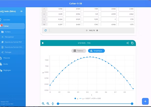
The experiment notebook is the central space where you organize your data, graphs, and observations. All measurements (audio, video, simulations, sensors) are automatically added to it.
8.2 Structure of the notebook
The notebook is organized into numbered observations:
- Each observation can contain data, graphs, images, and text
- Observations can be reordered by drag-and-drop
- Click + Add to insert an observation into the document
8.3 Content types
- Data tables: raw measurement data
- Graphs: visualization of relationships between quantities
- Images: screenshots, photos, spectrograms
- Text: comments, analyses, conclusions
- Formulas: mathematical equations (see document editor)
8.4 Working with data
- Variable selection: choose which columns to display
- Calculated columns: add derived quantities (formulas)
- Sorting and filtering: organize the data
- Copy-paste: to Excel, Google Sheets...
8.5 Graphs
Graphs are generated automatically from the data:
- Curves: time evolution, relationships between quantities
- Scatter plots: discrete data
- Histograms: statistical distribution
Graph options
- Selection of the X and Y axes
- Linear or logarithmic scale
- Adding trend lines (modeling)
- Legend and title
8.6 Modeling and curve fitting
FizziQ Web lets you fit mathematical models to the data:
| Model | Equation | Use |
|---|---|---|
| Linear | y = ax + b | Uniform motion, Ohm's law |
| Quadratic | y = ax² + bx + c | Free fall, projectile |
| Exponential | y = a·ebx | Radioactive decay, RC |
| Sinusoidal | y = A·sin(ωt + φ) | Oscillations, waves |
| Power | y = a·xn | Power laws |
9. Tables and graphs - Analyze
Captured data is represented as tables. Each table contains columns called quantities (time, distance, velocity...) and lets you view, edit, or enrich the experimental data.
9.1 Accessing tables
Table in the experiment notebook:
Each time you capture data (audio analysis, video, simulation, external sensor...), a table is automatically created in the experiment notebook. You can open it to view and edit the data.
Create a blank table:
- Open your experiment notebook
- Click + → Data table
- Enter your data manually
9.2 Quantities (columns)
Each column represents a quantity with:
- Name: e.g. Time, Distance, Velocity
- Unit (optional): in parentheses (m, s, m/s...)
- Type: manual entry or calculated
- Decimals: 0 to 6 for the display
Create a quantity: Click + new quantity to the right of the columns.
9.3 Entering data
Accepted formats:
- Whole numbers:
42,-15 - Decimals:
3.14or3,14(comma converted automatically) - Scientific notation:
1.5e-3,6.02e23
Navigation: Tab (right), Shift+Tab (left), Enter (confirm and move down), Esc (cancel).
9.4 Formulas
All formulas begin with = and use column names as variables.
Operators
| Operator | Example |
|---|---|
+ - * / | =Distance/Time |
^ (power) | =v^2 |
| Implicit multiplication | =0.5mv² is equivalent to =0.5*m*v^2 |
Mathematical functions
| Function | Description | Example |
|---|---|---|
sin(x), cos(x), tan(x) | Trigonometry (radians) | =sin(angle) |
asin(x), acos(x), atan(x) | Inverse functions | =atan(slope) |
sqrt(x) | Square root | =sqrt(distance) |
ln(x), log(x) | Natural and base-10 logarithms | =ln(concentration) |
exp(x) | Exponential e^x | =exp(-t/tau) |
abs(x) | Absolute value | =abs(delta) |
Constants: pi (3.14159...), e (2.71828...)
Statistical functions
| Function | Description |
|---|---|
somme(column) or sum(column) | Sum of the entire column |
moyenne(column) or average(column) | Mean of the column |
ecartype(column) or stdev(column) | Standard deviation of the column |
Differentiation functions
| Function | Description | Example |
|---|---|---|
diff(y, x) | First derivative dy/dx | =diff(position, time) → velocity |
diff2(y, x) | Second derivative d²y/dx² | =diff2(position, time) → acceleration |
Note: the first and last rows display #N/A (not enough points).
Reference to other rows
| Function | Description |
|---|---|
prec(column) or prev(column) | Value of the previous row |
suiv(column) or next(column) | Value of the next row |
Example: =position - prec(position) calculates the difference between two measurements.
9.5 Graphs
Click the graph icon in the toolbar to switch between table and graph.
Configuration (3 tabs)
Data tab:
- X axis: choose a column or "Index" (1, 2, 3...)
- Y axes: add up to 5 curves
Display tab:
| Marker type | Description |
|---|---|
| Circles only | Points without lines (default) |
| Circles + lines | Connected points |
| Lines only | Continuous curve |
| Interpolation | Equation | Use |
|---|---|---|
| Linear | y = ax + b | Linear law, proportionality |
| Degree-2 polynomial | y = ax² + bx + c | Free fall, parabola |
| Degree-3 polynomial | y = ax³ + bx² + cx + d | Complex curves |
| Exponential | y = a × e^(bx) | Radioactive decay, RC |
| Power | y = a × x^b | Power law |
Scales tab: Automatic adjustment or manual scales (Min/Max).
9.6 Integration with Python
Define functions in the Python interpreter and use them in the tables:
# In Python
def energie_cinetique(m, v):
    return 0.5 * m * v * v

# In the table (column formula)
=energie_cinetique(mass, velocity)
9.7 Import/Export
- CSV export: Export button → file with semicolon separator
- CSV import: Open button → automatic format detection
- Export to notebook: copies the table as a new observation
- Graph export: PNG or insertion into the editor
9.8 Error messages
| Message | Meaning |
|---|---|
#N/A | Value not available (normal for diff() at the edges) |
#ERR:COL | Column not found (check the spelling) |
#ERR:POINTS | Not enough points for diff() |
#ERR:VALEUR | Cell does not contain a number |
9.9 Keyboard shortcuts
| Shortcut | Action |
|---|---|
| Tab / Shift+Tab | Next / previous cell |
| Enter | Confirm and move down |
| Ctrl+Z / Ctrl+Y | Undo / Redo (50 actions) |
| Ctrl+C / Ctrl+V | Copy / Paste |
| Del | Clear the content |
10. Final report - Share
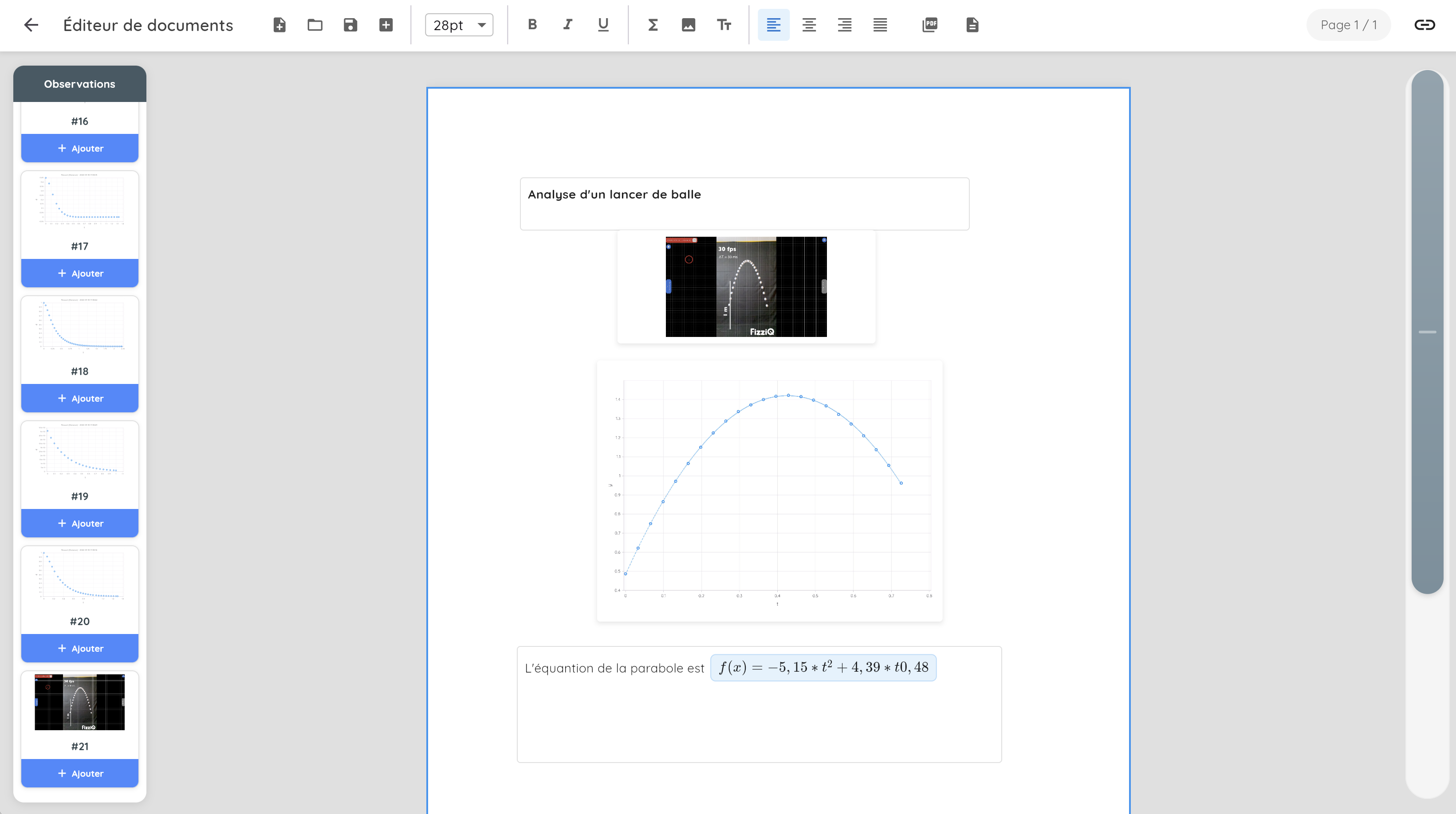
The final report is the third pillar of FizziQ Web: Share. After capturing data (Experiment) and organizing and understanding it (Analyze), the student can now communicate their results by creating a complete scientific document.
The FizziQ Web report editor is designed to be simple and effective. The student can:
- Write formatted text (headings, bold, italic...)
- Insert images and photos
- Directly integrate the cards from their experiment notebook (tables and graphs)
- Add mathematical formulas in LaTeX syntax
- Export the report to PDF, Word, or image to share it with the teacher
Creating a report is done in two steps:
- Enrich the experiment notebook: add text and photos, organize the cards
- Create the final report: format it with the text editor, then export
10.1 Enriching the experiment notebook
Before creating the final report, enrich your experiment notebook with explanatory text and photos.
Adding text to a card
- Open the relevant card in the experiment notebook
- Click Edit at the top right of the card
- Write your text in the text area
- Click Confirm to save
Adding photos
- From the experiment notebook, click + Add an observation
- Select Photo
- Choose an image from your computer or take a photo with the webcam
- Optionally add descriptive text
Editing the title of a card
- Click the title of the card
- Edit the text
- Press Enter to confirm
Organizing the cards
The cards appear in the report in the order in which they are arranged in the notebook:
- Move: drag a card to change its position
- Delete: click the trash can to remove an unneeded card
- Duplicate: create a copy to make variations
10.2 Accessing the report editor
- From the experiment notebook, click Edit the report
- Or go to Share → Final report
10.3 Editor interface
The report editor consists of three areas:
- Central area: the report being written
- Left sidebar: three buttons to insert elements
- Contextual toolbar: appears when text is selected
Sidebar: the 3 insertion buttons
| Button | Function | Description |
|---|---|---|
| Text | Add a text area | Inserts an empty text block that you can edit freely |
| Image | Insert an image | Opens a selector to choose an image from your computer |
| Observations | Integrate from the notebook | Displays the list of cards from the experiment notebook. Click a card to insert it into the report. |
10.4 Formatting the text
Select text to bring up the contextual toolbar:
- Font size: from 8pt to 72pt
- Bold (B): makes the text bold
- Italic (I): makes the text italic
- Alignment: left, center, right, justified
- Formula (Σ): inserts a LaTeX mathematical formula
10.5 Inserting mathematical formulas
FizziQ Web supports LaTeX syntax for scientific formulas. Two insertion methods:
Method 1: Σ button (recommended)
- Place the cursor at the desired location
- Click the Σ button in the toolbar
- Enter your formula in LaTeX syntax
- Click Insert
Method 2: Direct syntax with $...$
Type directly in the text:
$E = mc^2$for an inline formula- The formula is automatically converted into a mathematical rendering
Examples of LaTeX formulas
| LaTeX code | Result | Use |
|---|---|---|
E = \frac{1}{2}mv^2 | E = ½mv² | Kinetic energy |
T = 2\pi\sqrt{\frac{L}{g}} | T = 2π√(L/g) | Pendulum period |
\Delta t = t_2 - t_1 | Δt = t₂ - t₁ | Time interval |
a = \frac{dv}{dt} | a = dv/dt | Acceleration |
F = ma | F = ma | Newton's second law |
v = \sqrt{v_x^2 + v_y^2} | v = √(vx² + vy²) | Magnitude of the velocity |
\lambda = \frac{c}{f} | λ = c/f | Wavelength |
\frac{a}{b} for fractions, \sqrt{x} for square roots, x^2 for exponents, and x_i for subscripts.
10.6 Inserting images
- Click the Image button in the sidebar
- Select an image from your computer
- The image is inserted at the cursor position
- Resize it by dragging the corners if necessary
Useful image types:
- Photos of the setup: experimental assembly
- Screenshots: simulations, measurements
- Diagrams: explanatory drawings
- Chronophotographs: motion analysis
10.7 Integrating notebook observations
- Click the Observations button in the sidebar
- The list of all your notebook cards is displayed
- Click the desired card to insert it
- The table, graph, and text are automatically added
10.8 Structure of a scientific report
A quality scientific report generally includes:
| Section | Content |
|---|---|
| Title | Name of the experiment, date, author(s) |
| Objective | What you are trying to demonstrate or measure |
| Protocol | Description of the setup and method (with photo/diagram) |
| Measurements | Raw data tables (from the notebook) |
| Graphs | Visual representation of the results |
| Analysis | Interpretation, calculations, curve fitting, formulas |
| Uncertainties | Discussion of the sources of error |
| Conclusion | Validation or not of the hypothesis, answer to the research question |
10.9 Finalizing the report
Before exporting, you must finalize your report:
- Check that all the elements are correctly placed
- Reread the text to correct any errors
- Click the Finalize button
10.10 Exporting the report
Once finalized, several export formats are available:
PDF export (recommended)
- Click Export to PDF
- The PDF file is generated and downloaded
- Ideal for printing and sharing by email
Word export (.docx)
- Click Export to Word
- A .docx file is generated
- You can open and edit it in Microsoft Word, Google Docs, or LibreOffice
FizziQ file (.fiz)
The .fiz file contains all of your work:
- The complete experiment notebook
- All the tables and graphs
- The final report
- The inserted images
- Go to Share → Export the file
- A .fiz file is downloaded
- This file can be re-imported into FizziQ Web to continue the work
10.11 Frequently asked questions about the report
Can I edit the report after finalizing it?
Yes, click Unfinalize to return to edit mode. You will have to finalize again before you can export once more.
How do I change the order of the elements in the report?
Click an element and drag it to the desired position. You can also reorganize the cards in the experiment notebook before inserting them.
My LaTeX formula does not display correctly
Check the LaTeX syntax. Common errors are: missing braces, a forgotten backslash before commands (\frac, \sqrt...), or extra spaces.
Is the PDF export of good quality for printing?
Yes, the generated PDF is high-resolution, suitable for paper printing.
Can I insert several graphs from the same card?
When you insert an observation, all the associated graphs are automatically included. To insert only one, duplicate the card in the notebook and delete the unwanted graphs.
How do I add a caption below an image?
Insert a text area just below the image, reduce the font size, and center the text to create a caption.
Does the report keep the colors when exported?
Yes, the colors of the graphs, text, and images are preserved in the PDF and Word exports.
11. Exporting data - Share
FizziQ Web lets you export data at three levels:
- A single observation: export an individual card from the notebook
- The complete notebook: export the entire set of observations
- The final report: export the summary document
11.1 Exporting an observation (notebook card)
From the experiment notebook, you can export each observation card individually:
- Open the observation card in the notebook
- Click the Export button
- Choose the export format
Formats available for an observation
| Format | Description | Usage |
|---|---|---|
| CSV | Spreadsheet file (.csv) | Open the data in Excel, Google Sheets, LibreOffice |
| Python | Python script (.py) | Advanced analysis with numpy, matplotlib |
| Image | PNG image | Save a graph or a table |
| QR Code | QR code containing the data | Transfer the data to FizziQ on a smartphone |
Python export
The Python export generates a script containing:
- The data as numpy arrays
- The code to generate the graphs
- The curve fits
11.2 Exporting the complete experiment notebook
To export the entire experiment notebook:
- Scroll all the way to the top of the experiment notebook
- Click the Export button
- Choose the export format
Formats available for the complete notebook
| Format | Description | Usage |
|---|---|---|
| PDF document with all the observations | Printing, archiving. Layout options (number of columns...) | |
| FizziQ file | .fizziq file | Complete backup, later re-import into FizziQ Web |
11.3 Exporting the final report
To share all of your experimental work, use the final report:
- Create your report by integrating the notebook observations
- Click Finalize
- Choose the export format
Formats available for the report
| Format | Description | Usage |
|---|---|---|
| PDF document | Printing, sending by email, archiving | |
| Word | Word document (.docx) | Editing in Microsoft Word, Google Docs, LibreOffice |
11.4 Export summary
| Level | Access | Formats |
|---|---|---|
| A single observation | Export button on a card | CSV, Python, Image, QR Code |
| Complete notebook | Export button at the top of the notebook | PDF, FizziQ file |
| Final report | Finalize then Export | PDF, Word |
11.5 Privacy
12. Additional tools
12.1 Scientific calculator
A full calculator for quick computations:
- Basic operations (+, -, ×, ÷)
- Scientific functions (sin, cos, tan, log, exp...)
- Physical constants (π, e, c, g...)
- Calculation history
12.2 Sound synthesizer
Generate sounds at precise frequencies:
- Frequency: 20 Hz - 20,000 Hz
- Waveform: sine, square, triangle, sawtooth
- Volume: adjustable
- Beats: two simultaneous frequencies
Educational uses
- Study of audible frequencies
- Beat phenomenon
- Tuning instruments
- Doppler effect (with movement of the source)
12.3 Color synthesizer (RGB)
Mix the primary colors of light:
- RGB sliders: Red, Green, Blue (0-255)
- Display: resulting color
- Codes: RGB and hexadecimal values
Educational uses
- Additive color synthesis
- Color coding in computing
- Complementary colors
12.4 Video → chronophotograph converter
Transform a video into a chronophotographic image:
- Load a video
- Define the interval between frames
- Choose the number of frames to superimpose
- Adjust the transparency
- Export the resulting image
12.5 Python interpreter
A built-in Python environment for advanced analyses:
- Code editor: syntax highlighting
- Libraries: numpy, matplotlib available
- Data import: access to the notebook data
- Export: graphs and results to the notebook
Example script
import numpy as np
import matplotlib.pyplot as plt

# Notebook data
t = np.array([0, 0.1, 0.2, 0.3, 0.4])
y = np.array([0, 0.05, 0.20, 0.44, 0.78])

# Quadratic fit
coeffs = np.polyfit(t, y, 2)
print(f"Acceleration: {2*coeffs[0]:.2f} m/s²")

# Graph
plt.plot(t, y, 'o', label='Measurements')
t_fit = np.linspace(0, 0.4, 100)
y_fit = np.polyval(coeffs, t_fit)
plt.plot(t_fit, y_fit, '-', label='Fit')
plt.xlabel('Time (s)')
plt.ylabel('Position (m)')
plt.legend()
plt.show()
12.6 Screen sharing
Project FizziQ Web for the whole class:
- Full-screen display
- Presentation mode
- Synchronization with the students' devices
13. Settings
The settings let you configure and customize FizziQ Web to suit your needs: language, accessible tools, advanced parameters, and configuration sharing.
13.1 Accessing the settings
In the left sidebar, click Settings. The settings home page presents three sections:
| Section | Description |
|---|---|
| Language | Choose the interface language |
| Customization | Configure the accessible tools (restricted mode) |
| Parameters | Adjust the advanced parameters |
13.2 Changing the language
FizziQ Web is available in 21 languages: French, English, Spanish, Portuguese, German, Italian, Dutch, Swedish, Norwegian, Danish, Finnish, Hungarian, Estonian, Polish, Romanian, Ukrainian, Russian, Turkish, Arabic, Malagasy.
- In the settings, click Language
- Select the desired language from the list
- The interface updates automatically
13.3 Customization (Restricted mode)
Restricted mode lets teachers simplify the interface for their students by displaying only the tools needed for an activity.
Two display modes
| Mode | Description |
|---|---|
| Show all | All tools are accessible (default mode) |
| Custom mode | Only the selected tools are visible |
Enabling custom mode
- In the settings, click Customization
- Click Custom mode
- Check the tools to make accessible
- Uncheck the tools to hide
Available tools
General: Experiment notebook, My notebooks, Final report
Experiment: Audio Analysis, Video Analysis, Chronophotograph, External Sensors, Data Entry
Simulations: Waves on a lake, Ballistics, Centrifuge, Pendulum, Inclined plane, Spring, Electrical circuit, Ideal gas, Optics, Three-body
Tools: Text editor, Spreadsheet, Python, Calculator, Sound synthesizer, Color synthesizer, Video chronophotograph
13.4 Sharing a configuration
Teachers can generate a link so that their students access a custom configuration directly.
- Configure Custom mode with the desired tools
- Click Generate a link
- Copy the link with the Copy button
- Share the link with your students (email, learning platform, QR code...)
When a student opens the link, FizziQ Web loads automatically with the custom configuration.
13.5 Advanced parameters
In the settings, click Parameters to access the advanced options.
Kinematic fitting (quadratic)
- Enabled: Velocity and acceleration calculations use a quadratic interpolation over 3 points (recommended)
- Disabled: Calculation by simple finite differences
USB connection speed (Baud Rate)
Configures the communication speed with external USB sensors (FizziQ Connect, Arduino).
| Baud Rate | Description |
|---|---|
| 9600 | Very slow, very stable |
| 57600 | Fairly fast |
| 115200 | Fast (recommended, default value) |
| 230400 - 921600 | Very fast to maximum |
In case of problems: Corrupted data → lower the Baud Rate. Data too slow → raise the Baud Rate.
13.6 Configuring the AI assistant
FizziQ Web includes an AI assistant to help users. In the settings, expand the AI Chat section to configure:
| Model | Description |
|---|---|
| OpenAI GPT-5 mini | Fast, concise, efficient |
| Mistral AI Small | European model, detailed and thorough |
13.7 Saving the settings
13.8 Typical configurations for teachers
| Type of lab | Recommended tools |
|---|---|
| Mechanics | Video Analysis + Spreadsheet + Final report |
| Acoustics | Audio Analysis + Spreadsheet + Final report |
| External sensors | External Sensors + Spreadsheet + Final report |
| Simulation | A simulation + Spreadsheet + Final report |
14. Troubleshooting
14.1 Common problems
| Problem | Solution |
|---|---|
| The microphone does not work | Allow access to the microphone in the browser settings (padlock in the address bar) |
| The camera does not work | Allow access to the camera, close other applications using it |
| Bluetooth not available | Use Chrome or Edge, check that Bluetooth is enabled on the computer |
| The simulations are slow | Close the other tabs, check the computer's performance |
| Empty PDF export | Check that the notebook contains data, use the document editor |
| FizziQ Connect not detected over USB | Use a data USB cable, close Arduino IDE |
| Video does not load | Check the format (MP4, WebM recommended), file size |
| LaTeX formulas do not display | Check the syntax, use the provided examples |
14.2 Recommended browsers
For an optimal experience:
- Chrome (version 89+): all features
- Edge (version 89+): all features
- Firefox: audio, video, simulations (no Bluetooth/USB)
- Safari: audio, video, simulations (no Bluetooth/USB)
14.3 Chromebook
FizziQ Web works perfectly on a Chromebook:
- Use Chrome (installed by default)
- All features are available
- Ideal for institutions equipped with Chromebooks
14.4 Performance
If the application is slow:
- Close unnecessary tabs
- Clear the browser cache
- Reduce the size of the imported videos
- Limit the number of points in the simulations
14.5 Support
For any question: info@fizziqlab.org
Complete documentation: fizziq.org/post/documentation-fizziq-web
Appendix: Connecting microcontrollers
This appendix details how to program a microcontroller (Arduino, ESP32, micro:bit...) to transmit sensor measurements to FizziQ Web via USB. The microcontroller sends lines of text in a specific format that FizziQ Web recognizes automatically.
A.1 Compatible hardware
Any microcontroller with a USB port or a USB serial port:
- Arduino: Uno, Nano, Mega
- ESP32 or ESP8266
- micro:bit
- Teensy
- Raspberry Pi Pico
A.2 USB format expected by FizziQ Web
Each line of data must follow this format:
FZ[CHANNEL]:[LABEL]:[VALUE]Example messages
FZ0:tem:25.3
FZ0:hum:65.2
FZ1:pre:1013.25
FZ2:lum:450
Structure of a message
| Element | Description | Example |
|---|---|---|
FZ | Mandatory prefix | FZ |
[CHANNEL] | Channel number (0 to 5) | 0, 1, 2... |
[LABEL] | Abbreviation of the sensor type | tem, hum, lum... |
[VALUE] | Measured numeric value | 25.3 |
A.3 Recognized sensor labels
FizziQ Web recognizes these standardized abbreviations (not case-sensitive):
| Label | Quantity | Unit |
|---|---|---|
tem | Temperature | °C |
pre | Atmospheric pressure | hPa |
hum | Relative humidity | % |
lum | Brightness | lux |
acc | Acceleration | m/s² |
dis | Distance | mm |
son | Probe temperature | °C |
co2 | Carbon dioxide | ppm |
o2 | Oxygen | % |
ph | pH | - |
uv | UV index | UV |
tvo | Total VOCs | ppb |
inf | Infrared temperature | °C |
wei | Mass | kg |
ten | Electrical voltage | V |
int | Electrical current | A |
mag | Magnetic field | mT |
pou | Pulse | bpm |
rot | Rotation | rpm |
niv | Sound level | dB |
pm2 | PM2.5 particles | µg/m³ |
cv | Conductivity | mS/cm |
wat | Power | W |
an | Analog signal | - |
ext | Custom measurement | - |
A.4 Using multiple channels
FizziQ Web handles 6 channels (0 to 5) to distinguish several sensors of the same type:
FZ0:tem:25.3    // Temperature sensor 1
FZ1:tem:22.1    // Temperature sensor 2
FZ2:tem:28.5    // Temperature sensor 3
A.5 Serial port configuration
For a stable USB connection:
- Baud rate: 115200 (recommended)
- Data bits: 8
- Stop bit: 1
- Parity: none
A.6 Programming an Arduino
First test with a fixed value
void setup() {
  Serial.begin(115200);
}

void loop() {
  Serial.println("FZ0:tem:25.3");
  delay(1000);
}
Example with a real sensor (DHT22)
#include <DHT.h>

#define DHTPIN 2
#define DHTTYPE DHT22

DHT dht(DHTPIN, DHTTYPE);

void setup() {
  Serial.begin(115200);
  dht.begin();
}

void loop() {
  float temp = dht.readTemperature();
  float hum = dht.readHumidity();

  if (!isnan(temp)) {
    Serial.print("FZ0:tem:");
    Serial.println(temp, 2);
  }
  delay(100);

  if (!isnan(hum)) {
    Serial.print("FZ0:hum:");
    Serial.println(hum, 1);
  }
  delay(400);
}
Example with multiple sensors
#define TEMP_PIN A0
#define LIGHT_PIN A1

void setup() {
  Serial.begin(115200);
}

void loop() {
  int rawTemp = analogRead(TEMP_PIN);
  int rawLight = analogRead(LIGHT_PIN);

  float temperature = rawTemp * (5.0 / 1023.0) * 100.0;
  float lux = map(rawLight, 0, 1023, 0, 1000);

  Serial.print("FZ0:tem:");
  Serial.println(temperature, 2);
  delay(100);

  Serial.print("FZ0:lum:");
  Serial.println(lux, 1);
  delay(400);
}
A.7 Programming an ESP32
#define TEMP_PIN 34
#define LIGHT_PIN 35

void setup() {
  Serial.begin(115200);
}

void loop() {
  int rawTemp = analogRead(TEMP_PIN);
  int rawLight = analogRead(LIGHT_PIN);

  float voltage = (rawTemp / 4095.0) * 3.3;
  float temperature = voltage * 100.0;
  float lux = map(rawLight, 0, 4095, 0, 1000);

  Serial.print("FZ0:tem:");
  Serial.println(temperature, 2);
  delay(100);

  Serial.print("FZ0:lum:");
  Serial.println(lux, 1);
  delay(400);
}
A.8 Programming a micro:bit
JavaScript (MakeCode)
basic.forever(function () {
    let temp = input.temperature()
    serial.writeLine("FZ0:tem:" + temp)
    basic.pause(100)

    let lum = input.lightLevel()
    serial.writeLine("FZ0:lum:" + lum)
    basic.pause(400)
})
Python (micro:bit)
from microbit import *

while True:
    print("FZ0:tem:" + str(temperature()))
    sleep(100)
    print("FZ0:lum:" + str(display.read_light_level() * 4))
    sleep(400)
A.9 Recommended sending frequency
| Interval | Quality |
|---|---|
| 500 - 1000 ms | Ideal for most uses |
| 100 - 500 ms | Acceptable |
| < 100 ms | Too fast, risk of data loss |
| > 5000 ms | Too slow, choppy graph |
A.10 Connecting to FizziQ Web
- Plug the microcontroller into the computer with a data USB cable
- Upload your program (Arduino IDE, PlatformIO, MakeCode...)
- Close the programming environment
- Open FizziQ Web in Chrome or Edge
- Click Experiment → External sensors
- Click USB Serial
- Select the port corresponding to the microcontroller
- The detected sensors appear automatically
A.11 Microcontroller troubleshooting
| Problem | Possible causes | Solutions |
|---|---|---|
| No data appears | Incorrect format, missing FZ prefix, incorrect baud rate | Check the format, use Serial.println(), test with a fixed value |
| Inconsistent values | Faulty conversion, uncalibrated sensor, electrical noise | Reread the sensor documentation, check the wiring |
| Missing messages | Sends too fast, serial buffer full | Increase the sending interval, insert delays between data |
| USB port does not open | Arduino IDE open, another application using the port | Close all serial applications, change the USB cable |
| Microcontroller restarts | Insufficient power supply, short circuit | Check the power supply and the assembly |
A.12 Activity example: weather station
Build a small weather station with a microcontroller and a few sensors:
- Temperature sensor
- Humidity sensor
- Light sensor
The program sends:
FZ0:tem:23.4
FZ0:hum:58.1
FZ0:lum:420
In FizziQ Web, students can:
- Visualize the measurements in real time
- Record the data over a period of time
- Plot evolution graphs
- Compare different experimental conditions
- Export the data for analysis
# are ignored by FizziQ Web and can be used for debugging:
Serial.println("# Sensor initialized");
Serial.println("# ERROR: Sensor not found");